[Reading Note] Self-Supervised Learning from Images with a Joint-Embedding Predictive Architecture

Archived

Type: paper-review
Date: Sep 09, 2026
Read time: 20 min
Research field: Self-supervised Learning, Computer Vision
Methods: Joint-Embedding Predictive Architecture (JEPA)

Paper Information

Title: Self-Supervised Learning from Images with a Joint-Embedding Predictive Architecture

Authors: Mahmoud Assran, Quentin Duval, Ishan Misra, Piotr Bojanowski, Pascal Vincent, Michael Rabbat, Yann LeCun, Nicolas Ballas

Affiliation: Meta AI (FAIR), McGill University, Mila – Quebec AI Institute, New York University

arXiv ID: arXiv:2301.08243

Topic: Self-Supervised Learning, Joint-Embedding Predictive Architecture (JEPA), Representation Learning, Vision Transformer, Masked Prediction, Image Understanding

Venue: CVPR 2023 (IEEE/CVF Conference on Computer Vision and Pattern Recognition)

Pages: 15619–15629

① 왜 latent space에서 예측하는가, ② context/target/predictor는 각각 무엇을 하는가, ③ 왜 target block을 크게 잡는가, ④ 왜 EMA target encoder가 필요한가, ⑤ 이것이 MAE와 본질적으로 무엇이 다른가

1. One-line Summary

I-JEPA는 pixel reconstruction이나 hand-crafted augmentation invariance에 의존하지 않고, 보이는 context로부터 가려진 영역의 abstract representation을 예측함으로써 high-level semantic representation을 효율적으로 학습하는 self-supervised learning framework이다.

2. Problem

CV에서 Image SSL에 대한 두가지 연구 방향

Invariance-based method

같은 이미지에서 임의 크기 조정, 자르기, 색 jittering 등 손수 데이터 증강을 한 두세장의 이미지 뷰를 수집해 이에 대한 비슷한 임베딩을 생성하는 encoder를 최적화한다.

⇒ 하지만 이러한 방법들은 강한 bias도 함께 도입하며, 그 bias는 특정 downstream task나 서로 다른 데이터 분포를 사용하는 pretraining task에서는 오히려 불리하게 작용할 수 있다


⇒ 그리고  서로 다른 추상화 수준을 요구하는 task의 경우 이러한 편향들을 어떻게 일반화할 수 있는가 또한 아직 구체적으로 정해지지 않았다.


strong augmentation prior에 의존적이다.

Generative Method

인지 학습 이론에서는 생물학적 시스템에서 표현학습을 이끄는 핵심 매커니즘 중 하나가 감각 입력에 대한 반응을 예측하도록 내부 모델을 적응시키는 과정이라고 제안해왔다.

prediction→internal representation learning


Mask denoising과 같은 방법론은 임의로 마스킹된 패치를 입력값으로부터 토큰 수준이던 픽셀 수준이던 재현하는 방식을 통해 representation을 학습해왔다.

- 이 방식은 view invariance approaches보다는 사전 지식이 덜 요구되고 image modality를 넘어 일반화하기도 쉽다.
- 그 결과 얻어지는 representation은 일반적으로 **semantic level이 더 낮고,** linear probing과 같은 **off-the-shelf 평가**나, semantic classification task에서 supervision이 제한된 transfer setting에서는 invariance-based pretraining보다 성능이 떨어진다.
    - **off-the-shelf evaluation**은 보통 **backbone을 크게 손대지 않고 바로 representation quality를 평가**하는 설정
    - **lower semantic level은** representation이 더 **저수준 시각 정보**에 치우쳐 있다는 말
    - **limited supervision transfer setting은** 사전학습한 모델을 다른 task로 옮겨 쓸 때, **새 task의 라벨 데이터가 충분하지 않은 상황**
    - invariance-based pretraining은 서로 다른 augmentation을 적용한 두 입력이 있어도 **같은 semantic content라면 비슷한 representation을 만들도록 학습하는 방식**

        ⇒ 입력 형태는 달라도 의미가 같으면 representation은 같아야 한다.


⇒ 결국 전이학습에서 이전 방법론의 성능을 완전히 보려면 end-to-end fine-tuning과 같은 involved adaptation을 적용해야한다.

기존 self-supervised learning 방법들은 각각 한계를 가지고 있으며, 저자들은 사람이 설계한 image transformation에 포함된 추가적인 prior knowledge에 의존하지 않고도 self-supervised representation의 semantic level을 높이는 방법을 탐구한다.

- `extra prior knowledge encoded through image transformations`는 보통 **augmentation에 포함된 사전 가정**
    > 이런 변형 (crop, color jutter, blur,…)을 거쳐도 semantic identity는 유지된다.

Representation Learning에서의 representation 구분

종류	주로 담는 정보	예시
Low-level representation	색, edge, texture, local pattern	CNN 초기 layer, ViT 초기 patch feature
Mid-level representation	part, shape, local structure	눈, 바퀴, 다리, object part
High-level semantic representation	object identity, category, scene meaning	dog, car, interaction, action
Global representation	이미지/영상 전체 의미	CLS token, global pooled feature
Local / Patch representation	특정 위치 또는 patch의 의미	ViT patch token
Spatial representation	위치와 공간적 관계	object A가 B의 왼쪽에 있음
Temporal representation	시간 변화, motion, dynamics	walking, collision, trajectory
Relational representation	객체 간 관계 및 interaction	person-riding-horse
Multimodal representation	서로 다른 modality의 공통 의미 (shared representation space)	CLIP image-text embedding
Latent predictive representation	직접 관측되지 않은 상태/미래/target의 추상 표현	I-JEPA, V-JEPA 계열

representation learning에서 흔히 원하는 것은 단순히 정보를 많이 보존하는 representation이 아니라, downstream task에 필요한 정보를 잘 구조화한 representation입니다.

⇒ self-supervised learning의 여러 방법은 결국 compatible한 representation pair를 가깝게 만들고 incompatible한 pair를 멀게 만드는 문제로 볼 수 있다

2.1. Background

Notion image

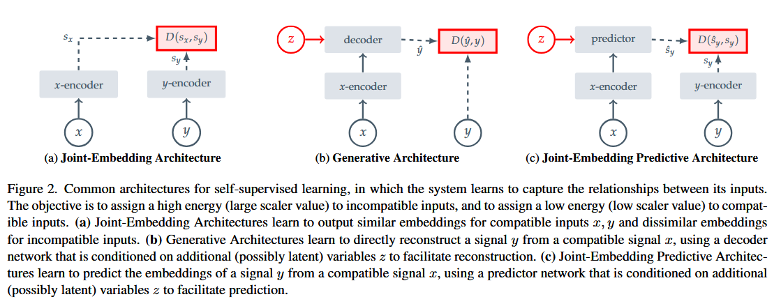
Source: Original Documentation

구조	$x$ 에서 무엇을 만드나	정답 target	loss가 계산되는 공간
JEA	$s_x$	$s_y$	representation space
Generative	$\hat y$	$y$	input/data space
JEPA	$\hat s_y$	$s_y$	representation space

2.1.1. Joint Embedding Architectures

Notion image

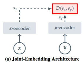
Source: Original Documentation - figure 2(b)

Invariance based pretraining은 Joint Embedding Architecture (JEA)를 활용한 Energy-Based Model의 한 종류라고 볼 수 있다

JEA란 무엇인가?

: compatible input $\bold x, \bold y$ 에 대하여 비슷한 임베딩을 생성하고 incompatible inputs에 대해서는 다른 임베딩을 생성하는 것을 의미한다.

Constrastive Learning과 어떤 관계인가?

: JEA는 두 입력을 같은 embedding space에 놓고 관계를 학습하는 구조이고, 여기에 같은 의미를 가진 쌍은 positive pair 다른 의미를 가진 쌍은 negative pair로 정의해서 positive→가깝게 negative→멀게 학습하도록 만든 것이 contrastive learning

JEA의 가장 큰 한계점 중 하나는 representation collapse인데 인코더가 입력값에 상관없이 항상 상수값을 생성하는 현상으로 energy landscape가 flat 하다고도 표현한다.

JEA에서 이 문제가 왜 생기냐,

기본 objective가 단순히 두 representation을 같게 만드는 것이라면

$z_x=f(x), \;z_y=f(y)$ 에 대해 $\|z_x-z_y\|^2$ 를 줄이려고 할 때 가장 쉬운 해답 중 하나가 $f(x)=f(y)=c$ 이기 때문

즉 모델이 의미를 학습하지 않고 그냥 **“모든 입력에 같은 벡터를 출력하면 둘이 항상 같네?”**라는 trivial solution을 찾게 된다. 이게 representation collapse

이 현상을 방지하기 위해 Contrastive Learning에서는 명시적으로 representation의 관계 (의미있는가, 없는가, 가까운가, 먼가)를 설정한다
Non-contrastive Learning에서는 아래와 같은 방법으로 collapse를 깬다

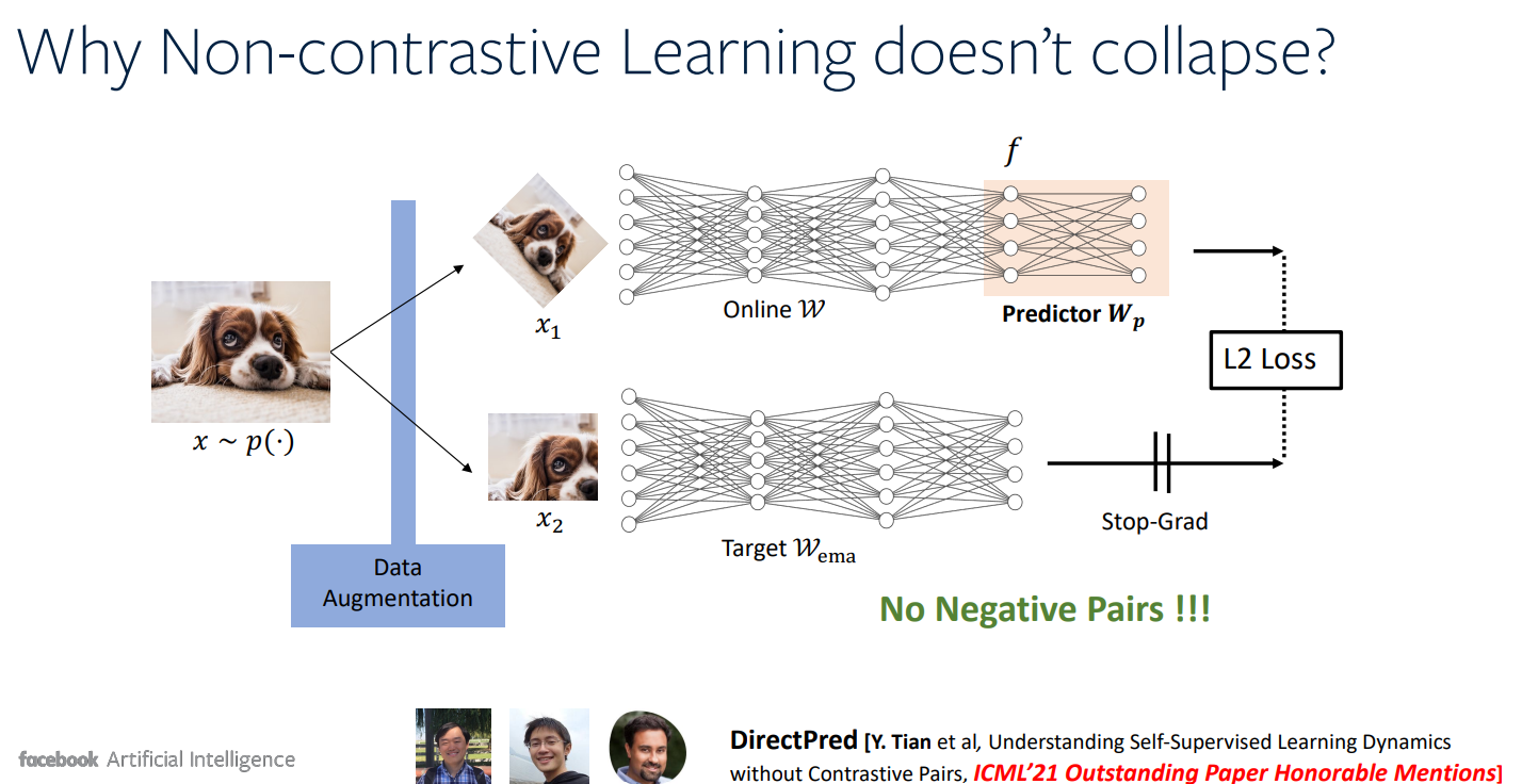
Source: Yuandong Tian, “Towards Better Understanding of Representation Collapsing in Representation Learning”, Meta AI, https://yuandong-tian.com/talks/talk_caltech_cs148.pdf
1. Source–target asymmetry
  
  : 두 branch를 완전히 동일하게 학습하지 않고 **역할을 다르게 두는 구조(Asymmetry)**한쪽은 예측하는 source/online branch, 다른 쪽은 예측 대상이 되는 target branch로 두어 두 네트워크가 동시에 같은 trivial solution으로 수렴하는 것을 막는다.
2. Predictor
  
  : source encoder가 만든 representation을 바로 target과 비교하지 않고, 추가 네트워크 $g_\phi$ 를 거쳐 target representation을 예측한다. $z_x \rightarrow g_\phi(z_x)=\hat z_y$
3. Stop-gradient / EMA target encoder
  
  : target branch를 source와 동일하게 gradient로 업데이트하지 않습니다. Stop-gradient는 target 쪽으로 gradient가 흐르지 않게 하고,
  
  source는 일반적인 gradient descent로 업데이트 : $\theta \leftarrow \theta - \eta \nabla_\theta L$
  
  target은 gradient로 업데이트하지 않고 source의 파라미터를 천천히 복사
  
  $\bar{\theta}\leftarrow\tau \bar{\theta}+(1-\tau)\theta$

2.1.2. Generative Architectures

Notion image

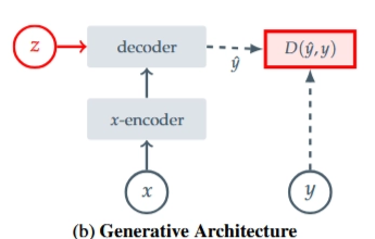
Source: Original Documentation - figure 2(b)

Reconstruction-based method는 EBM을 Generative Architecture로 구현한거다.

Generative Architectures란 compatible signal $x$ 로부터 신호 $y$ 를 바로 재구성한다. 그런데 이때 재구성을 돕는 추가적인 variable (주로 latent) $z$ 를 활용한 디코더 네트워크를 활용한다.

보통 compatible $x, y$ 를 생성하기 위해서 x는 y의 일부가 마스킹된 복사본으로 생성된다 (MAE)

⇒ 여기서는 $z$ 의 informational capacity가 signal $y$ 에 비해 낮은 이상 representation collapse가 발생하지 않는다.

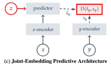
2.1.3. Joint-Embedding Predictive Architectures

Notion image

Source: Original Documentation - figure 2(c)

JEPA의 경우 Generative Architectures과 개념적으로 비슷하지만 loss function이 input space가 아닌 embiedding space에 적용된다는 것이다.

→ $y$ 신호의 임베딩을 compatiable signal $x$ 로부터 prediction을 보조하는 $z$ 를 추가적으로 활용해서 predictor network 상에서 예측하는 방식을 배운다.

Joint-Embedding Architecture와 달리, JEPA는 사람이 설계한 데이터 augmentation 집합에 대해 불변한 representation을 만들려고 하지 않는다. 대신 추가 정보 $z$ 가 주어졌을 때 서로를 예측할 수 있는 representation을 학습하려고 한다.

기존 prediction/reconstruction 기반 visual self-supervised learning은 다음과 같은 방향으로 발전해왔다.

Denoising autoencoders

입력에 noise나 masking 같은 corruption을 가한 뒤 원래 입력을 복원하도록 학습

$\tilde{x} \rightarrow x$ MAE도 이 계열의 현대적 형태
Context encoders

주변 context를 이용해 가려진 이미지 영역의 content를 직접 복원/regress

$x_{\text{surrounding}}\rightarrow\hat{x}_{\text{missing region}}$

context encoders / masked image modeling methods
Image colorization

grayscale image→color prediction

저자들의 목표는 downstream task에서 많은 양의 추가 fine-tuning 없이도 잘 작동하는 semantic representation을 학습하는 것

Our goal is to learn semantic representations that do not require extensive finetuning on downstream tasks

data2vec : The data2vec method learns to predict the representation of missing patches computed through an online target encoder (학습 과정 중에 target representation을 계속 새롭게 만들어내는 encoder)

> masked patch의 pixel이나 discrete token을 맞히는 것이 아니라, 학습 중인 teacher/target encoder가 full input에서 만들어낸 latent representation을 예측한다

Context Autoencoders : use an encoder/decoder architecture optimized via the sum of a reconstruction loss and an alignment constraint, which enforces predictability of missing patches in representation space.

⇒ 기존 방법들은 하나의 입력 이미지에 대해 여러 개의 augmentation view를 생성하고 각각을 네트워크에 통과시켜야 했기 때문에 계산량이 증가하고 scalability가 제한될 수 있었다. 반면 I-JEPA는 이미지당 하나의 view만 처리하면 되므로 더 효율적으로 확장할 수 있다

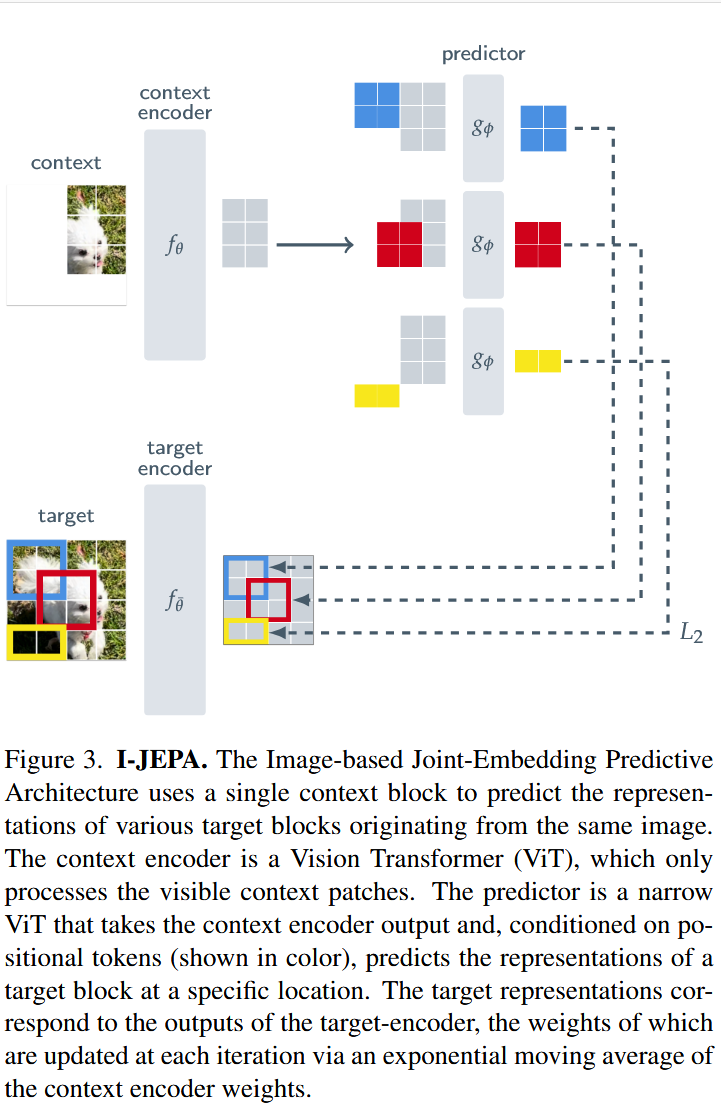
3. Method

sample target blocks with sufficiently large scale (semantic)
use a sufficiently informative (spatially distributed) context block

Notion image

Source: Original Document

MAE와 차이점은 I-JEPA의 경우 non-generative(data space에서 $y$ 를 생성 또는 복제하지 않는다)하며 prediction이 representation space에서 이루어 진다는거다.

3.1. Targets

입력된 이미지로부터 $N$ 개의 겹침없이 patch sequence로 만든 다음에 target-encoder $f_{\bar \theta}$ 에게 먹여 (feed) patch-level representation을 만든다.
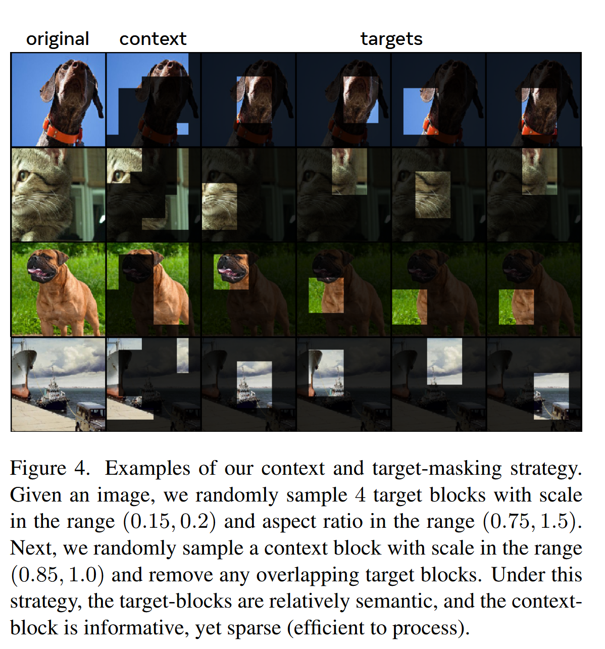
이런 patch-level representation에서 M개의 샘플을 겹치는 경우를 포함해서 추출하고 $B_i$ 로 기록한다. $s_y(i) = \{s_{y_i}\}_{j\in B_i}$ (저자들은 보통 4로 M을 설정하고 (0.75, 1.5) 사이의 random aspect ratio를 활용하고 (0.15, 0.2) 범위의 random scale을 활용했다고 한다.)

I-JEPA가 개별 patch 하나를 랜덤 선택하는 게 아니라, patch grid 위에서 직사각형 block 단위로 target을 샘플링한다
- random scale : 전체 이미지/patch grid 면적의 15~20% 정도를 차지하도록
- aspect ratio : 해당 block의 가로/세로 비율 → 실제 구현에서는 이 값을 patch grid 단위의 정수 width/height로 바꾼다.
  - Target encoder: 전체 이미지를 보고 좋은 정답 representation 생성
  - Context encoder: target 영역을 못 본 상태에서 그 representation을 예측
⇒ MAE는 입력 patch를 가리고 그 내용을 복원하지만, I-JEPA는 정답 representation 자체는 full image를 본 encoder가 만들어주고, context branch만 제한된 정보를 보게 한다.

→ 더 전체 맥락을 반영하는 representation을 생성할 수 있게 한다.

3.2. Context

I-JEPA의 목적은 단일 context block으로부터 target block representation을 예측하게 하는 것이다.

이미지로부터 85%~100%의 크기를 가진 단일 블록 $x$ $x$ 를 정사각형 비율로 표본추출한다.
- unit aspect ratio는 가로세로 비율이 1이라는 뜻
- $B_x$ : context block $x$ 와 관련된 마스크블록
target block은 context block과 독립 샘플링이 이루어지기 떄문에 overlap이 존재한다
ono-trivial prediction mask를 위해서 overlapping region의 경우 제거한다.

context block 안에 들어와 있던 target block과 겹치는 patch 영역을 context에서 제거한다.

$B_x'=B_x\setminus\left(B_{y_1}\cup B_{y_2}\cup \cdots \cup B_{y_M}
\right)$

![Notion image](/notion-assets/reading-note-self-supervised-learning-from-images-with-a-joint-embedding-predictive-architecture/3dc14b84a0f280939894d2d82067db51.png)


Source: Original Document

3. masked context block $x$ 가 context encoder $f_\theta$ 에 넣어 patch-level representation $s_x = \{s_{x_j}\}_{j\in B_x}$ 을 생성한다.

3.3. Prediction

context encoder로부터 출력된 $s_x$ 를 활용해 M개의 target block representation prediction을 진행한다.

target mask $B_i$ 에 대한 정답 representation $s_y(i)$ 에 대하여 predictor는 context encoder의 출력값인 $s_y(i)$ 를 입력값으로 받고 예측하기를 원하는 각각의 patch에 해당하는 mask token $\{m_j\}_{j\in B_i}$ 를 입력 값으로 받아
patch-level prediction $\hat s_y(i) = \{\hat s_{y_j}\}_{j \in B_i}$ 을 진행한다.
❓ mask token은 이때 어떤 역할을 수행하는가

모든 target patch에 완전히 다른 mask token을 두는 게 아니라, 기본 mask vector 하나를 공유하고 위치 정보만 다르게 붙인다
1. 학습 가능한 공통 mask vector를 하나 둔다. $m \in \mathbb{R}^d$
2. 이 $m$ 은 모든 target patch가 공통으로 사용해 아직 모르는 patch라는 공통 표현으로 활용한다.
이것만 쓰면 predictor는 각 mask token이 어느 위치를 가리키는지 구분할 수 없다.

그래서 각 위치 $j$ 마다 positional embedding $p_j$ 를 더한다. (ViT도 동일) $m_j = m + p_j$
- $m$ : “이 patch는 예측 대상이다”
- $p_j$ : “그리고 그 patch는 이 위치에 있다”

이 과정 predictor를 target block 수만큼 반복해서 적용한다

(predictor가 4개 따로 존재하는 게 아니라, 같은 predictor $g_\phi$ 를 재사용)

→ 달라지는 것은 각 실행에서 넣어주는 target 위치의 mask token

3.4. Loss

loss function은 두 representation 사이의 평균 L2 norm을 활용한다.

$\frac{1}{M}\Sigma_{i=1}^M D(\hat s_y(i), s_y(i)) = \frac{1}{M}\Sigma_{i=1}^M \Sigma_{j\in B_i} ||\hat s_{y_j}-s_{y_j}||^2_2$

Predictor $\phi$ 와 context encoder $\theta$ 의 경우 gradient-based optimization이 진행
target encoder $\bar \theta$ 의 경우 context-encoder의 exponential 이동 평균으로 업데이트된다.

ViT를 활용한 JEA 학습 과정에서 exponential moving average를 target-encoder에 적용하는건 증명이 되었기에 이를 그대로 사용했다고 한다.

⇒ EMA 방식의 target encoder가 JEA에서 그랬듯 I-JEPA에서도 학습 안정성과 collapse 방지에 매우 중요했다 (representation collapse 방지)

핵심은 target encoder를 gradient로 직접 빠르게 업데이트하지 않고

$\bar{\theta}\leftarrow\tau \bar{\theta}+(1-\tau)\theta$ 처럼 context encoder 파라미터의 이동평균으로 천천히 업데이트한다는 점입니다.

이렇게 하면 가장 큰 장점은 target representation이 너무 빨리 변하지 않는다는 것

4. Key Idea

learning highly semantic image representations without relying on hand-crafted data-augmentations.

⇒ from a single context block, predict the representations of various target blocks in the same image.

abstract representation에서 유실된 정보를 예측하게 한다.

e.g. 한개의 context block을 주고 같은 이미지 상에서 다양한 target block의 representation을 예측하게 한다. (이때 target representation은 이미 학습된 target-encoder 네트워크에서 계산한다)

단 I-JEPA는 pixel-level detail을 직접 복원하지 않고 abstract representation을 예측함으로써, downstream semantic task에 덜 중요한 저수준 정보를 제거하고 더 의미적인 특징을 학습하도록 유도한다.

I-JEPA에서 또 중요한 설계는 context block을 공간 적으로 분산되어 유의미한 정보를 담게하고 이를 활용해 image에서 충분히 큰 target block을 예측하게끔한다.

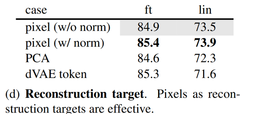
❓ target에 대한 연구는 이미 MAE에서 다루지 않았는가? 왜 이게 이 연구의 핵심이 될 수 있었을까

Source: Masked Autoencoders Are Scalable Vision Learners, 10.48550/arXiv.2111.06377

우선 MAE 연구에서는 정확하게 무엇을 이 테이블에서 비교한건가?

I-JEPA 연구에서는 무엇을 보고자 한건가?

MAE는 reconstruction을 통해 representation을 학습하고, I-JEPA는 representation 자체를 prediction target으로 삼아 semantic representation learning에 더 직접적으로 초점을 맞춘 구조

5. Result

Empirically, when combined with Vision Transformers, I-JEPA to be highly scalable

💡 Scalability라는 개념이 무엇이고 모델에서는 왜 중요한가?

Scalable하다 ⇒ 모델의 크기, 데이터 양, 학습 연산량을 늘렸을 때 성능이 계속 의미 있게 좋아지는 성질

CNN과 ViT는 어떤 차이가 존재하는가?

왜 논문들이 scalability를 중요하게 보는가?

현대 foundation model 연구에서는 결국 성능 개선의 큰 축이

만약 연구에서 방법론을 테스트할 때 ViT-S에서는 잘되는데 ViT-Huge에서는 성능 포화나 학습의 불안정성이 있다면 foundation model 방법론으로서는 한계가 존재하기 때문

Scalability: 모델·데이터·compute를 증가시켰을 때 성능이 지속적으로 향상되는 능력. 대규모 self-supervised/foundation model로 확장할 수 있는지를 판단하는 핵심 기준.

5.1. Image Classification

I-JEPA가 hand-crafted data-augmentation에 의존하지 않아도 high level representation 을 학습한다는 것을 증명하기 위해 linear probing과 partial fine-tuning protocol을 활용해 다양한 이미지 분류 태스크를 진행한다.

5.1.1. ImageNet-1K

IN1K에 사전학습된 Self-supervised model과 비교

Notion image

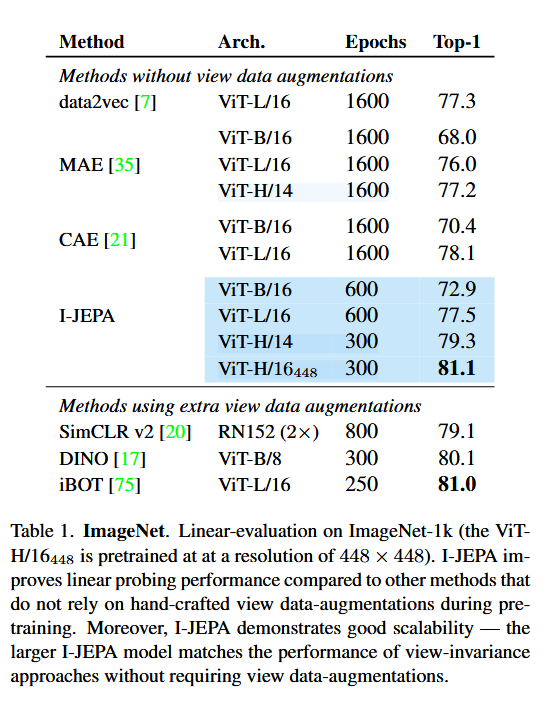
source: Original Document

Top-1 accuracy는 전체 샘플 중 정답 클래스를 맞힌 비율

Top-1 Accuracy=정답 클래스를 1순위로 예측한 샘플 수 / 전체 샘플 수

self-supervised pretraining 이후 model weight를 고정하고 linear classifier를 붙여서 IN1K에 학습시킨다.

⇒ I-JEPA가 linear probing 관점에서 다른 모델에 비해 성능을 향상시킨다는 것을 증명

pretrained representation 자체가 얼마나 class-separable하게 잘 정리되어 있는가

5.1.2. Low-Shot ImageNet-1K

Notion image

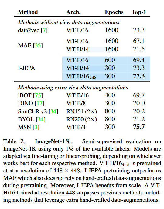
Source: Original Document

이번에는 1% ImageNet benchmark에 대해 성능을 측정했다.

ImageNet에서 self-supervised pretraining한 뒤, 전체 라벨의 1%만 사용하여 linear probing 또는 fine-tuning을 수행해 semi-supervised 성능을 평가했다.

Pretraining: ImageNet 이미지 사용, label 사용 X

Evaluation: ImageNet label 일부 사용

이는 클래스당 약 12~13장의 labeled image에 해당한다. 각 사전학습 방법에 대해서는 linear probing과 fine-tuning 중 더 높은 Top-1 accuracy를 기록한 결과를 보고했다.

zero-shot: 해당 downstream task의 라벨을 전혀 사용하지 않음

few-shot: 클래스당 몇 개처럼, 아주 적은 개수의 labeled sample만 사용

low-shot: 전체적으로 labeled data가 매우 적은 setting을 넓게 지칭

semi-supervised / low-label / low-shot transfer setting

pretrained representation이 이미 semantic하게 잘 정리되어 있어서 적은 supervision만으로도 downstream classification이 가능하다

5.1.3. Transfer Learning

Notion image

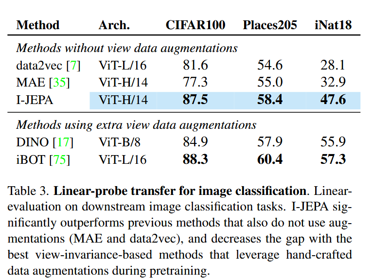
Source: Original Document

performance on various downstream image classification tasks using a linear probe.

이전에 나온 data augmentation을 활용하지 않는 방법 (MAE, data2vec)에 비해 좋은 성능을 보여주고 hand-crafted data augmentation을 요구하는 학습 방법과의 격차도 크게 줄였다.

5.2. Local Prediction Tasks

I-JEPA가 단순히 고수준 semantic representation만 잘 배우는지가 아니라, 공간적으로 세밀한 local information도 충분히 보존하는지를 검증한다.

Notion image

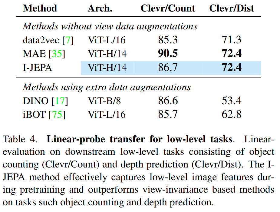
Source: Original Document

Clevr/Count: 이미지 안의 object 개수를 예측
Clevr/Dist: object의 depth/distance를 예측

DINO와 iBOT 같은 view-invariance 기반 방법보다 depth prediction에서 상당히 강했다. 다만 MAE보다 비등하거나 낮은 성능을 보여주었다.

5.3. Scalability

5.3.1. Model Efficiency

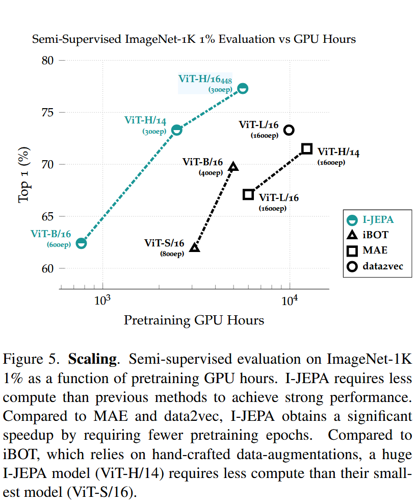
I-JEPA는 이전에 제시된 방법에 비해 scalable한가?

Notion image

Source: Original Document

GPU Hours의 증가에 따른 Top 1 accuracy를 검증했는데 I-JEPA 방법이 다른 방법에 비해 더 효율적인 학습을 했다는 것을 알 수 있다

물론 MAE는 pixel 을 직접적으로 target으로 활용하지만 I-JEPA의 경우 representation을 target에 대해 계산해야했기에 iteration 당 7% 정도 더 느렸다고 한다.
- 그럼 iteration 당 계산 속도는 느렸는데 어떻게 전체 효율은 I-JEPA가 더 높은 것인가?
  - Iteration efficiency=한 step이 얼마나 빠른가
  - Training Efficiency=원하는 성능까지 총 compute가 얼마나 필요한가
I-JEPA는 한 iteration 자체는 MAE보다 비쌀 수 있지만, 더 빠르게 유용한 semantic representation을 학습하기 때문에 같은 downstream accuracy에 도달하는 데 필요한 총 GPU hours는 더 적다.

5.3.2. Scaling data size

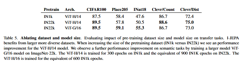
data size를 늘리면 성능 향상이 같이 이루어지는가?

Notion image

Source: Original Document

사전 학습되는 데이터셋의 크기를 늘리면 semantic, low level task 모두 성능이 향상됨을 볼 수 있다. (IN1K → IN22K)

5.3.3. Scaling model size

5.3.2. scaling data size와 마찬가지로 table 5를 achitecture에 대한 것으로 보면 모델의 크기가 클수록 (ViT-H/14 → ViT-G/16) 더 좋은 성능을 보여주었지만 low-level downstream tasks의 경우 오히려 성능이 떨어지는 (88.6 → 86.7) 모습을 보이기도 했다

5.4. Predictor Visualization

저자가 제시하는 I-JEPA predictor의 역할

context encoder의 출력 를 입력으로 받음 $s_x$
target block 위치를 나타내는 positional mask token을 조건으로 사용함
그 위치에 해당하는 target representation을 예측함

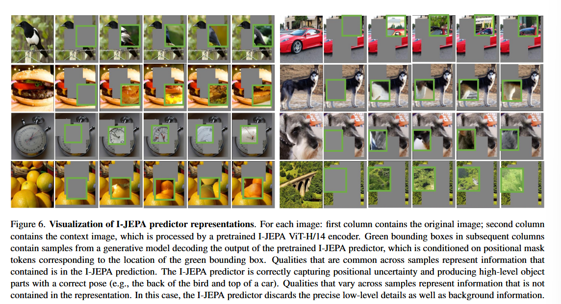
$\boxed{s^y=g_ϕ(s_x,\text{positional mask tokens})}$

저자들은 여기서 predictor가 단순히 위치 정보를 사용하는 것을 넘어**, 해당 위치에서 발생할 수 있는 target representation의 positional uncertainty**까지 적절히 학습할 수 있는지를 검증하고자 한다.

context+position 만으로는 확실히 예측 가능한 정보와 그렇지 않은 정보가 존재한다.

저자들은 predictor가 **“predictable high-level structure”**를 잡아내고, 예측 불가능한 low-level detail은 representation에서 덜 중요하게 만드는지를 확인

어떻게 실험 구조를 설계했는가?
1. I-JEPA 사전학습 후 context encoder와 predictor를 고정
  - 즉 representation 자체는 더 이상 바뀌지 않음
  - 이후 실험은 **이미 학습된 representation 안에 어떤 정보가 들어 있는가?**를 보기 위한 probe
- RCDM 방식의 decoder를 별도로 학습
  - predictor output을 average pooling하여 하나의 conditioning representation으로 만들고,
  - decoder가 그 representation을 조건으로 pixel-space 이미지를 생성하도록 학습
  - 중요한 점은 decoder가 I-JEPA를 다시 학습시키는 것이 아니라, frozen representation을 이미지로 시각화하기 위한 도구

Notion image

Source: Original Document

동일한 I-JEPA representation을 조건으로 stochastic decoder에서 여러 이미지를 샘플링했을 때, representation에 강하게 포함된 high-level semantic/spatial information(시계에는 초침과 분침이 있어야 하고 초침은 시침과 분침에 비해 얇다)은 반복해서 유지되지만, representation이 명확히 규정하지 않는 low-level detail(시간의 경우 지금 몇시인가?)은 샘플마다 달라진다.

❓ Representation-Conditioned Diffusion Model 어떤 pretrained representation을 조건(condition)으로 주고, 그 representation이 담고 있는 정보를 바탕으로 이미지를 생성하는 diffusion model

일반 diffusion model이 noise→image

RCDM은 noise+representation→image

5.5. Ablations Study

5.5.1. Predicting in representation space

Notion image

Source: Original Document

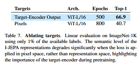
1% IN1K에 대한 low-shot performance를 비교했는데 조건은 pixel-space와 representation space 조건 상의 loss 계산 차이

⇒ representation 에서 계산하는게 훨씬 효과적이었고 이것이 I-JEPA의 중요한 요소였다.

왜 그런가?

저자들은 이에 대해 target encoder에게 abstract prediction target에 대한 예측 능력을 학습하게 하는 것이 불필요한 pixel-level detail을 제거해주는 효과를 얻었다고 한다.

5.5.2. Masking strategy

Notion image

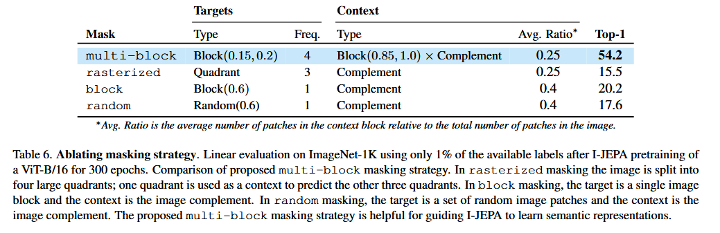
Source: Original Document

I-JEPA에서 활용한 multi-block masking 전략 외에도 다양한 방식을 활용해보고 성능을 비교한다.

rasterized: 벡터나 3D/도형 정보를 픽셀 격자의 이미지 형태로 변환한 것

예를 들어 선, 폴리곤, 지도 객체를 224×224 이미지의 픽셀값으로 바꾸면 “rasterized representation” raster = pixel grid

quadrant: 평면을 네 부분으로 나눈 사분면

좌표평면에서는 보통 1~4사분면을 뜻하고, 영상에서는 화면을 top-left / top-right / bottom-left / bottom-right 네 영역으로 나눴을 때 각각을 quadrant라고 부르기도 함

이 밖에도 마스킹 전략에서 범위 설정을 어떻게 진행할 것인가에 대해 서등 다른 요소에 대해서도 점검을 했다고 한다.

Notion image

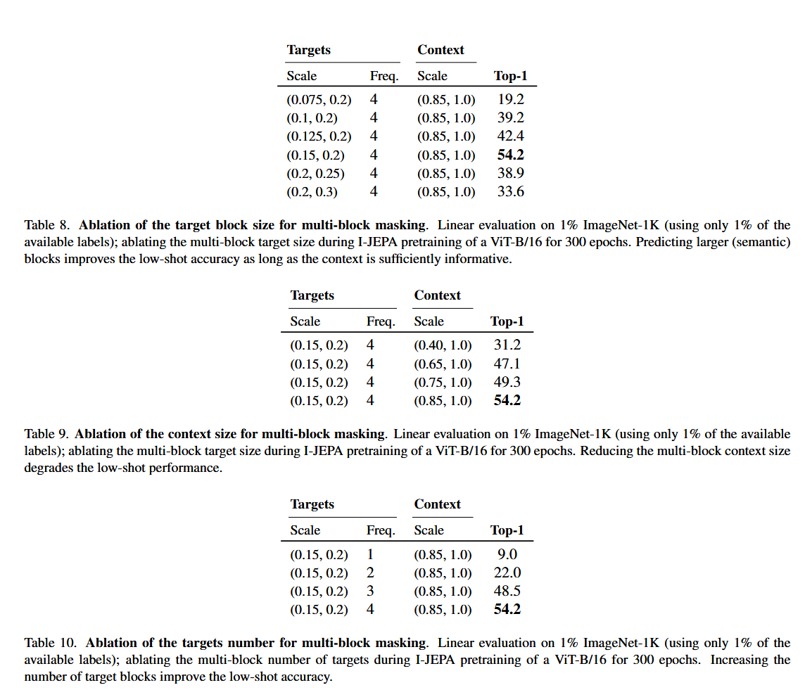
Source: Original Document

6. Limitation

정적 이미지 중심
- I-JEPA는 이미지 내부의 spatial context를 이용해 target representation을 예측합니다.
- 따라서 motion, temporal dynamics, causality 같은 시간적 정보는 다루지 못합니다.
Hand-crafted masking strategy에 의존
- augmentation에 대한 의존은 줄였지만, target block의 개수, scale, aspect ratio, context 크기 등은 사람이 설계합니다.
- 즉 prior가 완전히 사라진 것은 아닙니다.
Uncertainty를 명시적으로 모델링하지 않음
- predictor는 하나의 deterministic representation을 예측합니다.
- 여러 plausible target을 확률분포 $p(s_y\mid s_x,z)$ 형태로 직접 표현하지는 않습니다.
Semantic quality 평가가 간접적
- linear probing, low-shot classification, transfer, RCDM visualization 등을 통해 semantic representation의 품질을 추론합니다.
- representation 자체의 semantic level을 직접 정량화하는 명확한 지표는 없습니다.
추가 학습 구조 필요
- context encoder 외에도 target encoder와 predictor가 필요하고, target encoder는 EMA 방식으로 관리해야 합니다.
- 따라서 MAE처럼 단순한 encoder-decoder reconstruction 구조보다 학습 메커니즘이 복잡합니다.
Objective 자체의 효과 분리가 어려움
- 성능 향상이 latent prediction 자체 때문인지, $\text{large target block} + \text{EMA target encoder} + \text{predictor} + \text{ViT scaling}$ 의 조합 때문인지 완전히 분리해서 보기 어렵습니다.
범용성 검증의 한계
- ImageNet과 몇몇 downstream task에서는 좋은 결과를 보였지만, 강한 domain shift나 다양한 real-world structured prediction task에서도 항상 같은 장점이 유지되는지는 추가 검증이 필요합니다.