[Reading Note] Masked Autoencoders Are Scalable Vision Learners

Completed

Type: paper-review
Date: Aug 17, 2026
Research field: Self-supervised Learning, Computer Vision
Methods: Classification, Encoder–Decoder Architecture, Masked Autoencoder

Paper Information

Title: Masked Autoencoders Are Scalable Vision Learners

Authors: Kaiming He, Xinlei Chen, Saining Xie, Yanghao Li, Piotr Dollár, Ross Girshick

Affiliation: Facebook AI Research (FAIR)

arXiv ID: arXiv:2111.06377

Topic: Self-Supervised Learning, Masked Autoencoders (MAE), Vision Transformer (ViT), Visual Representation Learning, Image Reconstruction

Venue: IEEE/CVF Conference on Computer Vision and Pattern Recognition (CVPR 2022)

Pages: 16000–16009 (10 pages)

1. One-line Summary

High-ratio random masking과 asymmetric encoder-decoder를 통해 대규모 ViT를 효율적으로 self-supervised pre-training하고, 강한 transferable visual representation을 학습하는 MAE를 제안했다.

2. Problem

Large vision models → labeled data hunger → self-supervised learning 필요 → NLP의 masked modeling 성공 → 그런데 vision에서는 왜 덜 성공했는가? Deep learning has witnessed an explosion of architectures of continuously growing capability and capacity

capacity: 모델이 얼마나 많은/복잡한 패턴을 표현하고 학습할 수 있는가

→ 주로 모델 규모와 표현력

parameter 수

width/depth

모델이 fitting할 수 있는 함수의 복잡성

이 논문에서는 이후 ViT-Large, ViT-Huge 같은 큰 모델을 high-capacity models라고 부릅니다.

capability: 그 모델이 실제로 무엇을 얼마나 잘 할 수 있는가

→ 모델의 실제 능력이나 성능

이미지 인식 성능

다양한 downstream task로의 일반화

더 복잡한 문제를 처리하는 능력 등’

⇒ 모델은 점차 1M image 규모 가지고는 overfitting을 할 정도의 표현력을 갖추게 되었고 점차 더 많은 labeled image를 원하게 되었는데 이걸 public하게 구하기란 어려웠다.

⇒ NLP에서도 이 문제가 다뤄졌었는데 해결책은 GPT의 Autoregressive language modeling과 BERT의 masked autoencoding이었다.

> 두 방식은 공통적으로 **입력의 일부 정보를 모델에게 보이지 않게 한 뒤 이를 예측**함으로써 label 없이 학습한다.
- GPT: 미래 token을 보지 않고 다음 token을 예측
- BERT: 일부 token을 masking하고 해당 token을 예측

|        | Autoregressive                   | Masked Autoencoding                                         |
| ------ | -------------------------------- | ----------------------------------------------------------- |
| 대표     | GPT                              | BERT                                                        |
| 가리는 방식 | 미래 전체를 보지 않음                     | 일부 token을 선택적으로 mask                                        |
| 예측     | 다음 token                         | 가려진 token                                                   |
| 사용 문맥  | 이전 context                       | 양쪽 context                                                  |
| 강점     | 생성에 자연스러움                        | representation learning에 유리                                 |
| 대표 한계  | 미래 context 사용 불가, 생성이 sequential | mask와 실제 입력의 차이, 직접적인 생성에는 부자연스러움 (e.g. [MASK]와 같은 인위적인 토큰) |

그런데 NLP에 비해 vision의 autoencoding 발전이 뒤처져 있었다

다음의 관점에서 어떤 부분이 masked autoencoding이 vision 분야와 language 분야에서 다르게 만드는가? 에 대해 탐구

CNN에서는 mask token이나 positional embedding처럼 ‘특정 위치에 의미를 부여하는 별도 표시자(indicator)’를 자연스럽게 넣기 어렵다

⇒ 하지만 ViT가 이미지를 patch token sequence로 표현하면서 mask token이나 positional embedding 같은 token-level indicator를 자연스럽게 사용할 수 있게 되었으므로, 이러한 architectural gap은 더 이상 주요 장애물이 아니다.
정보의 밀도가 vision과 language는 다르다
- 언어는 인간이 생성한 신호로 맥락적인 정보가 많고 정보의 밀도도 높다.
  
  ⇒ 모델을 학습시킬 때 문장 당 몇개의 사라진 단어를 에측하는 데에도 세밀한 언어에 대한 이해가 필요하다.
- 이미지의 경우 객체나 장면의 의미를 깊게 이해하지 않고도 인접한 지역의 low-level statistics만 이용해 빈 부분을 맞힐 수 있다 (Spatial Redundancy)
  
  Spatial redundancy

    : 이미지의 인접한 영역들이 색상, texture, edge 등의 정보를 많이 공유하기 때문에 일부 patch가 없어져도 주변 정보만으로 쉽게 추정할 수 있는 성질.

⇒ 매우 높은 비율의 random masking을 통해 spatial redundancy를 크게 줄여, 주변 texture나 edge 같은 **low-level image statistics만으로는 해결하기 어려운** task를 만든다. 이를 통해 **모델이 object와 scene의 전체 구조를 고려하는 holistic understanding을 학습하도록 유도**한다.


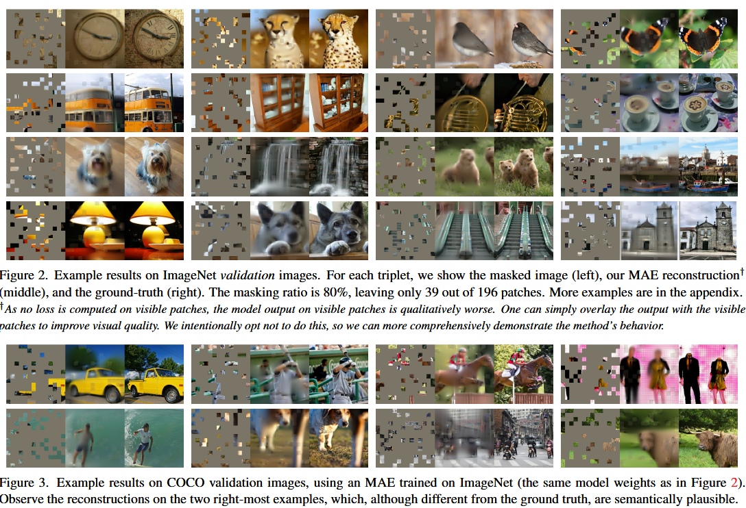
![Notion image](/notion-assets/reading-note-masked-autoencoders-are-scalable-vision-learners/3c114b84a0f280c99d17ed9501ff277c.png)


Source: Original Document

3. Autoencoder의 decoder는 latent representation을 다시 원래 입력 공간으로 매핑하는 역할을 하며, 텍스트와 이미지를 재구성할 때 그 역할이 서로 다르다. - Vision에서는 decoder는 pixel을 재구성하므로 최종적으로 맞혀야 하는 것은 의미적 개념이 아니라 pixel 값이다

    ```python
    낮은 semantic level
    ────────────────────
    Pixel value
    Color / edge / texture
    Local shape
    Object part
    Object
    Scene / concept
    ────────────────────
    높은 semantic level
    ```

- Language에서는 decoder가 의미적 개념인 단어를 예측하는거다.

⇒ 따라서 BERT에서는 디코더가 MLP로 구성되며 사소한 반면에 이미지에서는 디코더가 학습된 latent representation의 의미론적 수준을 정하는데 있어 핵심적인 역할을 한다.

    > 이미지 decoder의 output이 low-semantic-level이기 때문에 decoder가 더 단순해도 되는 것이 아니라, 오히려 그 **low-level reconstruction 작업이 encoder까지 침범하지 않도록** decoder가 reconstruction-specific processing을 충분히 담당해야 한다.

    ⇒  **[후속 Section 4.1의 설명과 연결]** **이미지 decoder가 reconstruction-specific processing을 충분히 담당**하면 **encoder의 latent representation을 보다 abstract한 수준**에 남겨둘 수 있다.

A. Masked Language Modeling

MLM과 autoregressive model은 NLP의 사전 학습 분야에서 이미 검증된 성공적인 방법론이었음

input sequence의 일부를 버리고 사라진 내용을 예측하게 하는 기법

⇒ scalability가 좋다

사전학습된 representation들은 특정 pre-training task에만 국한되지 않고 다양한 downstream task에도 잘 전이된다는 것이 많은 연구를 통해 확인되었다.

B. Autoencoding

입력은 latent representation을 매핑하고 디코더는 input을 재구성한다.

k-means, PCA도 autoencoder라고 함

💡 Denoising autoencoders (DAE) : a class of autoencoders that corrupt an input signal and learn to reconstruct the original, uncorrupted signal.

기본 Autoencoder:

Denoising Autoencoder:

⇒ MAE도 입력값에 corruption을 발생시킨다는 점에서 generalized DAE라고 볼 수 있다.

C. Masked image encoding

Context Encoder: 이미지의 큰 영역을 통째로 비워 놓고, CNN으로 그 부분을 채우는 방식

```plain text
Original Image
→ 큰 영역을 제거
→ CNN Encoder/Decoder
→ missing region inpainting
```

**iGPT:**이미지를 pixel sequence처럼 취급하며 unknown pixel을 예측한다

```plain text
Image pixels
→ pixel sequence
→ Transformer
→ 다음/가려진 pixel 예측
```

ViT의 masked patch prediction : ViT는 pixel 하나씩이 아니라 patch 단위로 처리

```plain text
Image
→ Patch 1, Patch 2, Patch 3, ...
→ 일부 patch masking
→ Transformer
→ masked patch 예측
```

MAE 논문은 이 ViT의 patch-based representation을 그대로 활용한다. 다만 MAE는 단순히 masked patch prediction을 하는 데서 끝나지 않고,
1. 매우 높은 masking ratio
2. masked patch를 encoder에 넣지 않는 구조
3. lightweight decoder
4. pixel reconstruction
를 결합한다.

BEiT: BEiT는 masked patch의 raw pixel 값을 직접 예측X, 대신 이미지를 먼저 별도의 tokenizer를 통해 discrete visual token으로 바꾼 뒤, 그 token의 ID를 맞히는 방식

대략:

Image patch
→ dVAE tokenizer
→ discrete token ID

예:
patch A → token 381
patch B → token 72
patch C → token 918

D. Self-supervised learning

pretext task: 정답 label 없이 representation을 학습하기 위해 인위적으로 만들어 놓은 사전학습 문제

contrastive learning: 이미지의 유사성만 학습하거나 유사성과 다른 점에 대해 학습하게끔 같은 이미지에서 다른 view를 만들어 학습하는 방식

⇒ Data augmentation에 의존하는 방식

>

**왜 data augmentation에 강하게 의존하는가?**


Contrastive 계열에서 `view` 자체를 보통 augmentation으로 생성한다.


```plain text
원본 사진
   ↓
View 1 = crop + flip + color jitter
View 2 = 다른 crop + color jitter
```


모델에게 **“겉보기에는 꽤 달라졌지만 둘 다 같은 이미지니까 같은 semantic representation을 가져야 한다.”**를 학습시키는 것.


그래서 augmentation이 학습 문제 자체의 핵심이다.


저자들은 뒤의 MAE ablation에서 이 차이를 실제로 다시 주는데, Contrastive learning은 augmentation이 없으면 두 view가 사실상 동일해져 **너무 쉬운 trivial problem**이 될 수 있다고 지적한다.

3. Method

visible patches → large encoder → latent representations → mask tokens 추가 → lightweight decoder → pixel reconstruction

💡 그럼 Decoder에 reconstruction 에 대한 학습을 넘겨주면서 어떤 이득을 취하는가? 만약 decoder가 너무 약하면,
Encoder
↓
"색, texture, edge, 세부 pixel 구조까지
내가 다 준비해야 함"
↓
아주 작은 Decoder
↓
Pixels
처럼 reconstruction에 필요한 세부적인 처리가 encoder representation에 더 많이 남을 수 있습니다.

반대로 decoder가 어느 정도 충분한 capacity를 가지면,
Encoder
↓
좀 더 abstract한 representation
↓
Decoder
├─ reconstruction-specific processing
├─ texture/detail 처리
└─ pixel-level prediction
↓
Pixels
처럼 reconstruction에 특화된 부분을 decoder가 담당할 수 있고, encoder의 latent representation은 보다 abstract한 수준에 남을 수 있다는 것이 저자들의 해석

MAE는 좋은 encoder representation을 얻는 것이 목적이므로, pixel reconstruction에 특화된 세부 처리를 decoder가 담당하게 하고 encoder의 latent representation은 상대적으로 더 추상적이고 recognition에 유용한 정보를 유지하도록 유도한다.

encoder that maps the observed signal to a latent representation
a decoder that reconstructs the original signal from the latent representation

이 autoencoder 구조는 이미 흔하지만, 이 논문에서는 비대칭적 (무거운 인코더와 가벼운 디코더) 구조를 활용해서 encoder는 마스킹되지 않은 부분에 대해서만, decoder는 full signal 복원을 수행한다.

Masking

이미지를 겹침 없는 패치로 나누고 그것들 중 일부분을 균등분포를 따른다는 가정 하에 중복없이 임의 추출한 뒤에 추출되지 않은 나머지를 마스킹하는 전략을 취함

⇒ 이때 상당수를 마스킹하는 전략은 정보의 중복 (image는 정보의 밀도가 낮기에 주변부가 모두 주어진다면 너무 쉽게 예측된다.) 을 막고 특히 균등 분포는 잠재적인 중앙 편향을 방지한다. (더 많은 마스킹된 패치들이 이미지 중앙으로 가는 현상. 정규분포의 종 모양을 생각하면 좋음)

Creating a task that cannot be easily solved by extrapolation from visible neighboring patches

MAE encoder

Encoder는 오직 visible한, 마스킹되지 않은 패치들에 대해서만 연산을 진행한다. (25% 정도의 소수)

⇒ 무겁고 큰 Encoder가 연산과 메모리 자원을 조금만 써도 학습할 수 있게 한다.

MAE decoder

Decoder는 Encoded visible patches와 mask tokens 두개를 모두 담는 전체 토큰을 입력 받는다.

각각의 마스킹된 토큰은 예측될 missing patch의 존재를 나타내는 shared, learned vector이다.

또한 마스킹된 토큰이 어디에 있을지에 대해 positional embedding을 모든 토큰에 대해 넣는다.

Decoder는 오직 사전 학습에만 사용되고 그러므로 decoder architecture는 encoder design에 대해 독립적으로 유연하게 설계 가능하다.

⇒ 그렇기에 저자들은 인코더에 비해 더 작고 좁으며 얕은 디코더들로 실험을 진행했는데, 전체 토큰은 오직 경량화된 디코더에 대해서만 적용되기 때문에 사전학습 시간을 크게 줄여준다.

Reconstruction target

MAE는 입력값을 재구성하는데 각 마스킹된 패치에 대해 pixel value를 예측하는 방식으로 진행한다. 디코더의 각 output token/element은 모두 patch를 나타내는 pixel 값들의 벡터로 이루어져 있고 마지막 층은 출력 채널의 수가 패치속 픽셀값의 수와 일치하는 linear projection을 진행한다.

⇒ Decoder output을 다시 patch 형태로 reshape하여 reconstructed image를 만들고, original image와 reconstructed image 사이의 MSE를 pixel space에서 계산한다.

⇒ 그런데 오직 masked pathes에 대해서 MSE를 계산한다 (BERT와 비슷한 방법론)

또한 저자들은 각 마스킹 된 패치의 normalized pixel value가 reconstruction target이게끔도 실험 설계를 해보았다.

특히 개별 patch 내부의 pixel vlaue에 대해 mean, standard deviation을 활용해서 normalization을 진행하였다.

⇒ 그랬더니 representation quality가 개선되었다고 한다.

Simple implementation

MAE의 사전학습은 별다른 특화된 연산 없이 효율적으로 구현된다고 한다.

모든 input patch에 대한 토큰을 생성하는데 added positional embedding과 함꼐 linear projection으로 생성한다.
토큰의 리스트를 임의로 순서를 섞고 마지막 부분을 제거하는데 이 제거되는 부분이 바로 masking ratio에 기반하여 제거한다.

⇒ 남는게 바로 input token for encoder가 된다. (비복원추출)

인코딩 뒤에 encoded patches 리스트에 mask token 리스트를 붙이고 이전에 했던 임의로 순서를 섞는 과정을 반대로 시행해서 모든 토큰이 target에 정렬되게 한다.

한 이미지의 patch sequence
[P0, P1, P2, P3, P4, P5]

↓ random shuffle 생성

ids_shuffle = [2, 5, 1, 4, 0, 3]

↓ 동시에 inverse index 계산

ids_restore = inverse(ids_shuffle)

디코더를 이 full list에 적용한다.

물론 이 shuffle/unshuffle 과정에서 발생하는 overhead가 있긴 하지만 무시할 수준(neglible)이라고 한다.

3. 1. Experiment Structure

ImageNet-1K의 학습 데이터셋을 활용해서 self supervised 사전학습을 진행한뒤

(i) end-to-end fine-tuning, (ii) linear probing 방식으로 representation을 평가하는 supervised training을 진행했다.

Baseline

ViT-Large (ViT-L/16)을 비교군으로 활용했는데 ViT-L의 특징으로는 ResNet-50보다 훨씬 큰 규모이며 그렇기에 overfit하는 경향이 있었다고 한다.

따라서 강한 regularization을 통해 ViT-L의 성능을 사전학습을 하지 않고 평가했지만 그래도 MAE의 성능이 더 높았다.

	Linear probing	End-to-end fine-tuning
Encoder	Freeze	Update
학습	Linear classifier만	Encoder + classifier 전체
보는 것	현재 representation의 linear separability	representation의 downstream adaptability / 전체 활용 가능성
질문	“지금 feature만으로 바로 분류 가능한가?”	“조정하면 얼마나 좋은 task model이 되는가?”
representation 수정	불가능	가능
장점	pre-trained feature 자체를 비교하기 쉬움	실제 downstream 활용 성능에 가까움
한계	nonlinear하게 좋은 feature를 과소평가할 수 있음	representation 자체와 fine-tuning 효과가 섞임

Notion image

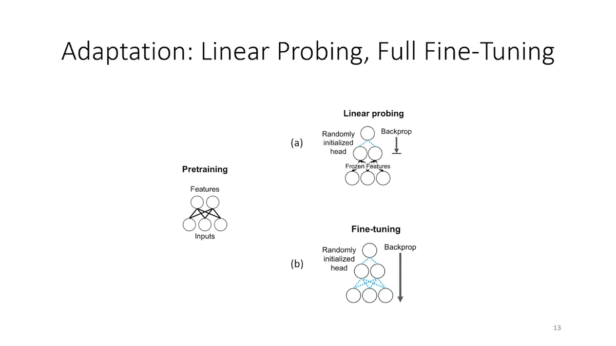
Source: Snorkel AI, Boost foundation model results with linear probing and fine-tuning (2023), https://snorkel.ai/blog/boost-foundation-model-results-with-linear-probing-fine-tuning/

Foundation Model을 활용할 때 사용하는 기법이기도 하다

핵심은 pre-trained feature를 유지할 것인가 (Linear Probing), 또는 초기값으로 활용할 것인가 (End-to-End Fine-tuning)

Source: Snorkel AI, Boost foundation model results with linear probing and fine-tuning (2023), https://snorkel.ai/blog/boost-foundation-model-results-with-linear-probing-fine-tuning/

Linear probing:

“Encoder가 이미 만들어 놓은 feature 자체에 class 정보가 얼마나 선형적으로 드러나 있는가?”

End-to-end fine-tuning:

“이 pretrained encoder가 downstream task에 맞게 조정될 때 얼마나 강력한 최종 representation/model로 발전할 수 있는가?”

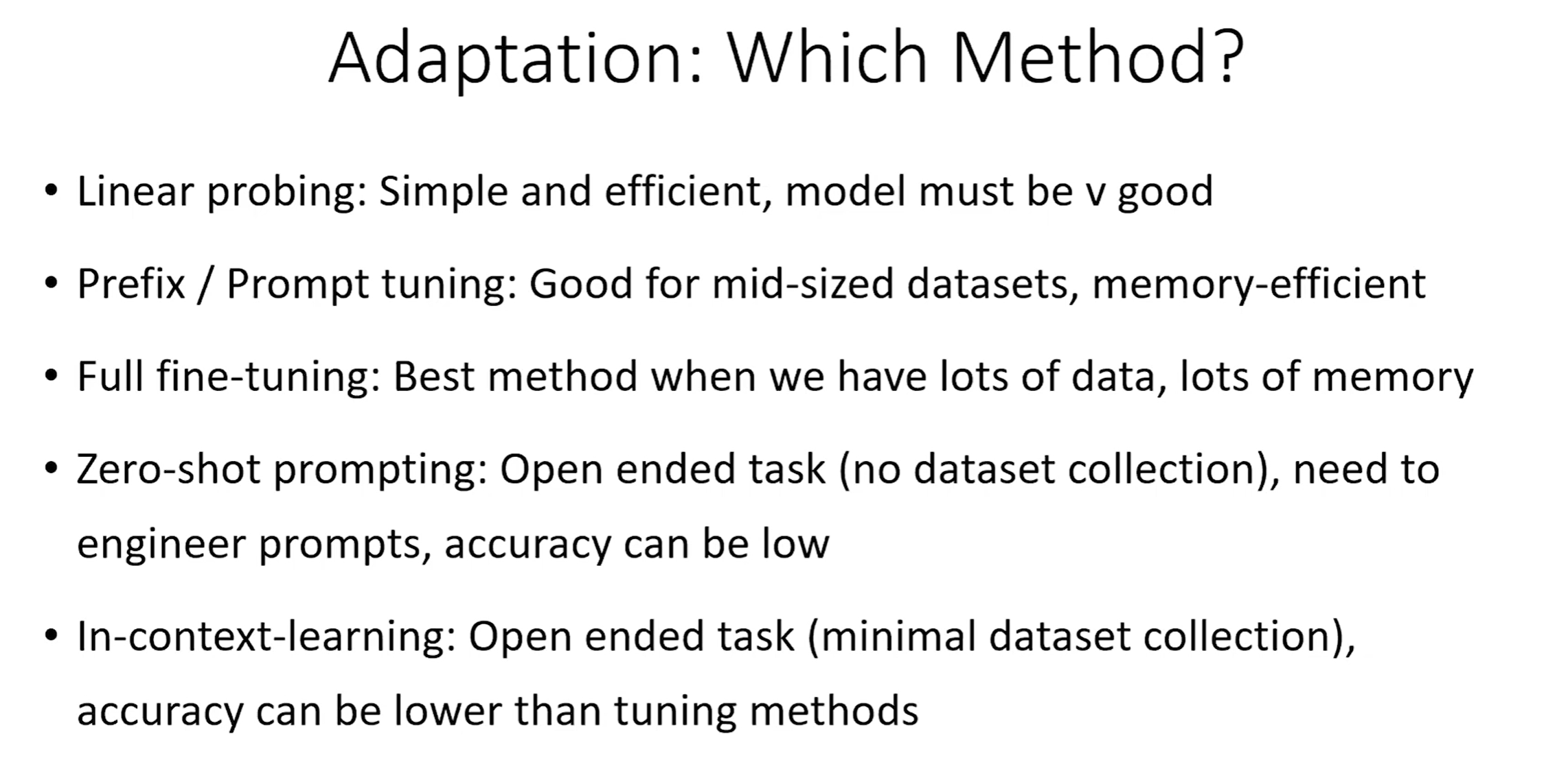
linear probing은 pre-training 결과를 더 직접적으로 검사하는 평가

평가	Encoder 수정	주로 보는 것
Linear probing	X	pre-trained feature의 직접적인 linear separability
Partial fine-tuning	일부	representation이 조금만 조정해도 유용해지는지
Full fine-tuning	전체	pretrained model이 최종 downstream task에 얼마나 잘 적응하는지

Notion image

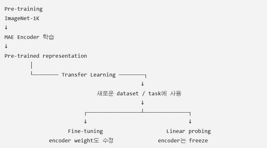
💡 Transfer Learning과 Fune-tuning은 개념적으로 어떻게 다른가?

Transfer learning

Fine-tuning

⇒ 좋은 representation은 반드시 처음부터 linearly separable할 필요는 없고, supervised signal을 조금 줬을 때 좋은 downstream solution으로 쉽게 변형될 수 있어도 좋은 representation

Notion image

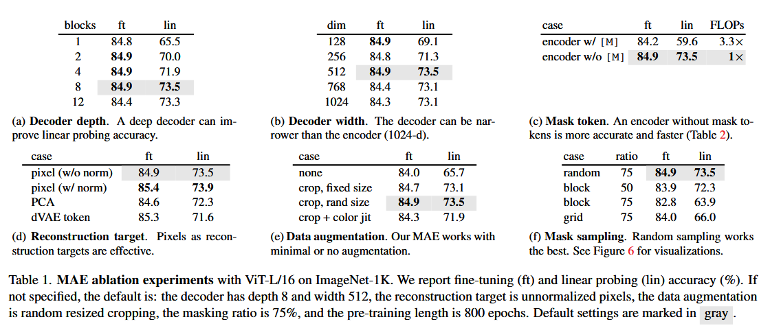
Source: Original Document

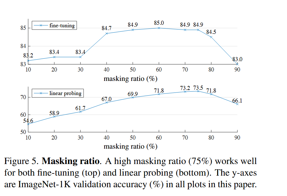
3.1.1. Masking Ratio

Notion image

Source: Original Document

Linear Probing과 Fine-tuning의 결과로 나오는 validation accuracy는 서로 연관되지 않은 모습을 보인다.

Linear Probing의 경우 특정 임계점 전까지는 꾸준하게 증가하고 상승 폭 또한 크다 (~20%)
반면 fine-tuning의 경우 차이가 그렇게 크지 않고 (~1%) masking ratio에 민감하지 않은 모습을 보인다.

3.1.2. Decoder Design

Notion image

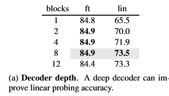
Source: Original Document Table 1, ft : fine-tuning, lin: linear probing

**decoder depth (number of Transformer blocks)**에 따른 Accuracy를 확인한게 위의 표이다.

> decoder depth는 validation 단계의 decoder가 아니라, **MAE self-supervised pre-training 과정에서 사용하는 decoder의 깊이**

linear probing에서는 디코더의 깊이가 충분히 깊어야 했는데 저자들에 따르면 pixel reconstruction task와 recognition task의 차이의 영향 때문이라고 한다.

설명을 보태자면 autoencoder의 마지막 층이 reconstruction에 더 특화되어있기 때문에 더 깊은 디코더가 reconstruction specialization에 더 특화된 작업을 수행 가능하게 된다

→ 그렇기에 인코더는 latent representation을 더 abstract한 수준으로 남길 수 있었다.
하지만 fine-utining의 경우 인코더의 마지막층이 recognition task에 조정될 수 있기 때문에 decoder의 깊이 자체는 문제가 되지 않았다.

정리

Decoder가 최소 1개의 Transformer block은 가져야 한다.

이것은 linear probing 때문이 아니다.

visible token의 정보를 mask token으로 전달하려면 self-attention이 최소 한 번은 필요하기 때문에 구조적으로 1 block이 최소 요건

Linear probing 성능을 좋게 하려면 decoder가 ‘충분히 깊은 것’이 중요했다.

1 block만으로는 reconstruction specialization을 decoder가 충분히 담당하지 못할 수 있다.

decoder를 어느 정도 깊게 하면 reconstruction-specific 처리를 decoder 쪽에 맡길 수 있고, encoder의 latent representation은 더 abstract한 수준

그래서 frozen encoder를 그대로 평가하는 linear probing에서 큰 차이가 난다.

Notion image

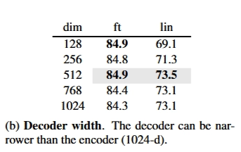
Source: Original Document Table 1, ft : fine-tuning, lin: linear probing

이번에는 Deocder의 width (channel 수)의 영향을 확인했다.

512 dimension을 기본값으로 했는데, linear probing과 fine-tuning에서 모두 성능이 좋게 나온 조건이기 때문이다.

더 좁은 decoder도 fine-tuning에서는 충분히 잘 작동한다 128-d나 256-d처럼 encoder보다 좁은 decoder도 fine-tuning에서는 거의 성능 저하 없이 잘 작동했다. 이는 narrow decoder가 더 우수하다는 의미라기보다는, decoder를 encoder만큼 넓게 만들 필요가 없다는 것을 보여준다. 기본 512-d decoder는 linear probing 성능과 계산 효율을 함께 고려한 선택

3.1.3. Mask token

Notion image

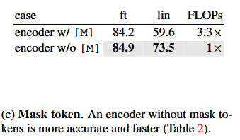
Source: Original Document Table 1, ft : fine-tuning, lin: linear probing

An important design of our MAE is to skip the mask token [M] in the encoder and apply it later in the lightweight decoder.

⇒ MAE의 중요 설계 중 하나는 mask token (M )을 encoder에서는 입력값으로 받지 않고 lightweight decoder에서만 입력값으로 받는다인데, 이게 효과가 있는지를 검증하겠다.

w/ : Mask Token을 Encoder에도 받아본 결과 비용측면에서도 악화되고 Accuracy 면에서도 약 14%p가 하락 (Linear Probing case)하는 결과가 나왔다.

저자는 아래와 같이 원인을 추측했지만 확정은 아님

_this encoder has a large portion of mask tokens in its input in pretraining, which does not exist in uncorrupted images. This gap may degrade accuracy in deployment._

w/o : Mask Token을 Encoder에는 제외하는 방식을 취한 결과 fine-tuning에서는 linear probing에 비해 성능 차이가 작았으나 (84.2 → 84.9) overall training FLOPs가 기존 대비 3.3× 감소한다 wall-clock 기준 2.8× speedup을 얻었다 (42.4h → 15.4h).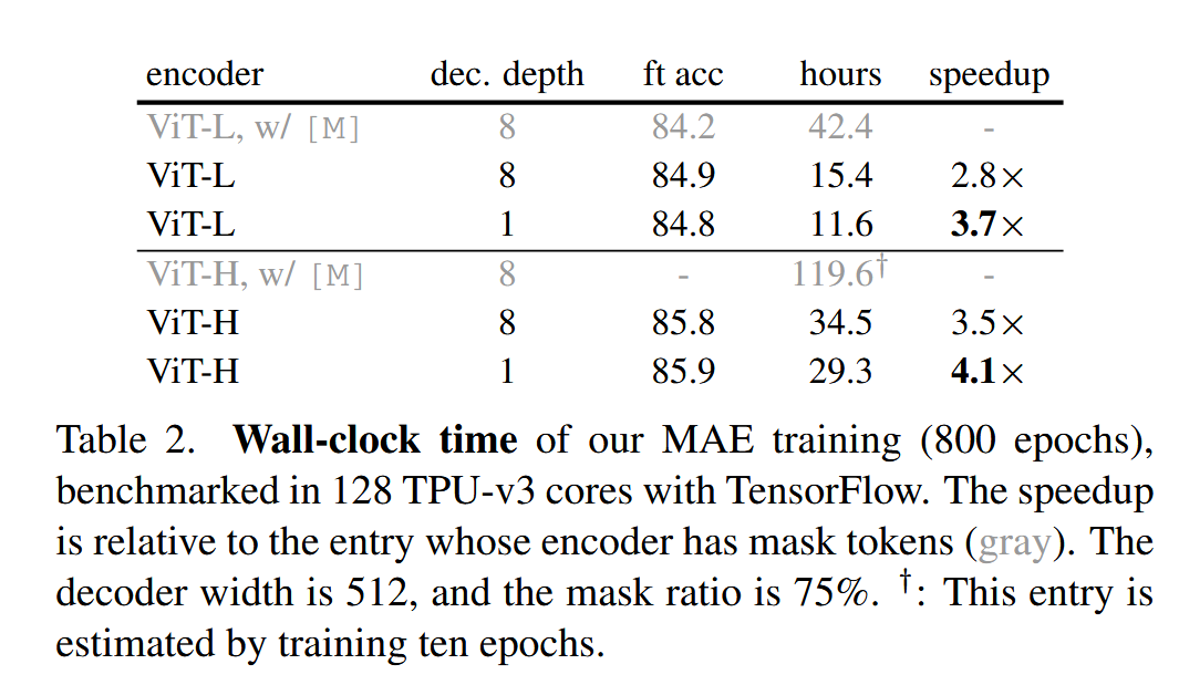

Source: Original Document
💡 FLOPs란? **FLOPs (Floating Point Operations)**는 모델이 연산을 수행하면서 필요한 부동소수점 연산의 양을 나타내는 계산 비용 지표

예를 들어 matrix multiplication에서 곱셈과 덧셈을 얼마나 많이 수행하는지를 대략 세는 것입니다.
```
FLOPs ↑ → 필요한 계산량 ↑ → 일반적으로 학습/추론 비용 ↑
```
다만 FLOPs는 실제 걸린 시간 자체는 아닙니다. GPU/TPU 성능, 메모리 접근, 병렬화 정도 등에 따라 같은 FLOPs라도 실제 시간은 달라질 수 있습니다.
💡 Wall-clock time이란? : 말 그대로 시계를 켜놓고 측정했을 때 실제로 학습에 걸린 시간입니다.

예를 들어 Table 2에서 ViT-L, decoder depth 8 기준으로:

설정 학습 시간
Encoder w/ mask tokens 42.4시간
Encoder w/o mask tokens 15.4시간

따라서 실제 학습 시간이 42.4→15.4 hours 로 줄었고, 저자들은 이를 2.8× speedup이라고 표현

즉:
- FLOPs = 이론적인 계산량
- Wall-clock time = 실제로 걸린 시간
Masking Ratio를 높이면 그만큼 self-attention 복잡도는 낮아지니 더 빨라지고 메모리 소비도 더 적어진다.

설정	학습 시간
Encoder w/ mask tokens	42.4시간
Encoder w/o mask tokens	15.4시간

3.1.4. Reconstruction target

Notion image

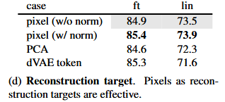
Source: Original Document Table 1, ft : fine-tuning, lin: linear probing

MAE가 masked patch를 복원할 때 무엇을 정답으로 맞히게 하는 것이 좋은 encoder representation을 만드는가?

⇒ normalization 을 한 pixel을 타겟으로 할 때 ft와 lin 모두 성능이 가장 높게 나온다.

테이블에서의 내용은 서로 다른 reconstruction target을 사용해 MAE를 새로 pre-train한 것
- pixel (w/o norm) : 원본 pixel 그대로 예측
- pixel (w/ norm) : patch별로 normalize한 pixel 예측 $x_{norm}=\frac{x−μ_{patch}}{σ_{patch}}$ $x_{n or m} = \frac{x - μ _{p a t c h}}{σ _{p a t c h}}$
  - 입력 이미지를 normalize하는 실험이 아니라 decoder가 맞혀야 하는 정답을 normalize한 것
- PCA : pixel 전체를 맞히지 말고 PCA representation을 예측
  - largest PCA coefficients 96개를 reconstruction target으로 사용
- dVAE token : pixel 대신 discrete visual token 맞히기
  - DALL-E에서 pre-trained된 dVAE tokenizer가 image patch를 discrete token ID로 변환합니다.
```
Image patch
↓
dVAE tokenizer
↓
Token ID = 827
```
    그러면 MAE decoder의 목표도 pixel 값이 아니라:
    
    이 masked patch의 token은 몇 번인가? → 827

“좋은 visual representation을 배우려면 decoder가 pixel처럼 low-level한 것을 직접 예측하는 것이 너무 단순하지 않은가? PCA나 semantic-like discrete token 같은 더 가공된 target이 낫지 않을까?

⇒ pixel level만으로 충분하다.

3.1.5. Data augmentation

Notion image

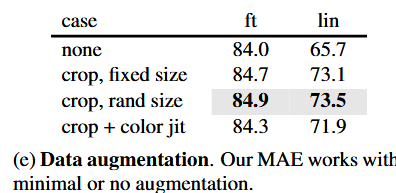
Source: Original Document Table 1, ft : fine-tuning, lin: linear probing

MAE pre-training 과정에서의 Data Augmentation의 효과 검증

색까지 변조를 주는 것 보다 cropping만 하는 것이 성능 향상에 도움을 주었다. 하지만 data augmentation 없이 (중앙 crop만 진행) 학습하는 것 또한 어느정도 좋은 성능을 보인다.

⇒ baseline이 비슷한 성능을 보이는 이 것이 contrastive learning 과 related methods에 비해 다른 점인데, 이 두 방법론의 경우 data augmentation에 의존적이기 때문이다

⇒ 그렇다면 MAE는 왜 data augmentation에 의존적이지 않았는가?

MAE에서는 random masking 자체가 매 iteration마다 새로운 corrupted input을 만들고 pretext task의 난이도를 높이는 일종의 regularization 역할을 한다. 따라서 contrastive learning처럼 다양한 view를 만들기 위한 강한 data augmentation에 크게 의존하지 않는다.

강한 masking
→ spatial redundancy 감소
→ 주변 patch만 보고 쉽게 복원하기 어려움
→ pretext task 난이도 상승
→ shortcut 학습 억제
→ 별도의 augmentation 필요성 감소

3.1.6. Mask sampling strategy

Notion image

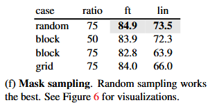
Source: Original Document Table 1, ft : fine-tuning, lin: linear probing

Mask sampling의 전략을 다르게 취한다면 모델 성능에 영향을 주는가?

완전 random 75%

block 단위로 50%

block 단위로 75%

공간적으로 붙어 있는 patch들을 큰 직사각형/블록 단위로 묶어서 제거하는 방식
1. 이미지 patch grid에서 어떤 시작 위치를 고르고
2. 일정한 높이와 너비를 갖는 block을 선택한 다음
3. 그 block 안의 patch들을 모두 mask하고
4. 원하는 masking ratio에 도달할 때까지 이런 block을 반복해서 선택
grid 모양으로 75%

Block으로 마스킹을 진행하는 경우 random 보다 더 어려운 과제가 되었는데, higher training loss가 관찰되었고 재생성된 결과도 뿌옇게 되었다.
- → block-wise는 너무 큰 연속 영역을 제거해서 75%에서는 과도하게 어려운 reconstruction task가 되었다

Notion image

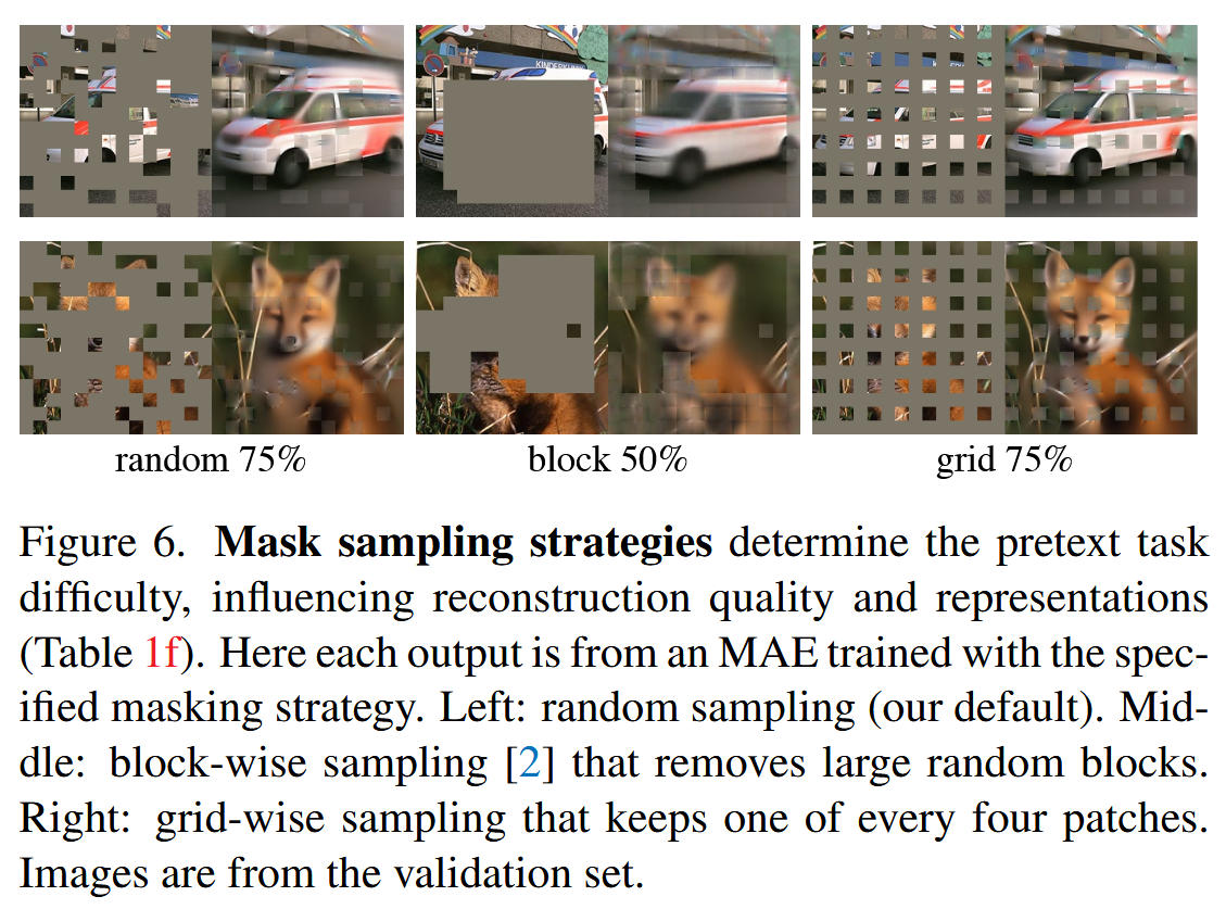
Source: Original Document

3.1.7. Training schedule

Notion image

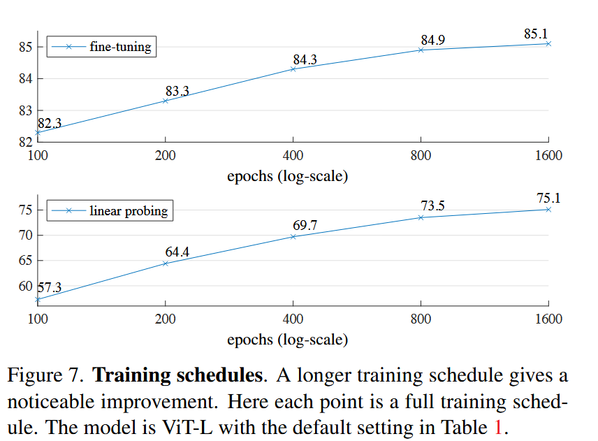
Source: Original Document

pre-training 단계에서 epochs를 늘리면 늘릴 수록 성능이 좋게 나오는가?

“동일한 ViT-L을 MAE로 더 오래 pre-train하면, 최종 encoder representation이 더 좋아지는가?”

→ 일단 실험 결과만 봤을때에는 steadily increase

contrasive learning method와 비교했을때 같은 ViT-L backbone을 사용하는 MoCo v3는 약 300 epochs에서 saturation되는 것과 다른 양상이다.

MAE는 전체 패치의 25%만을 epoch 당 보지만 contrastive learning의 경우 encoder가 200% 혹은 그 이상의 패치를 동일 epoch당 보는 것을 고려해야한다

4. Key Idea

High random masking (~75%) + Asymmetric encoder-decoder

Notion image

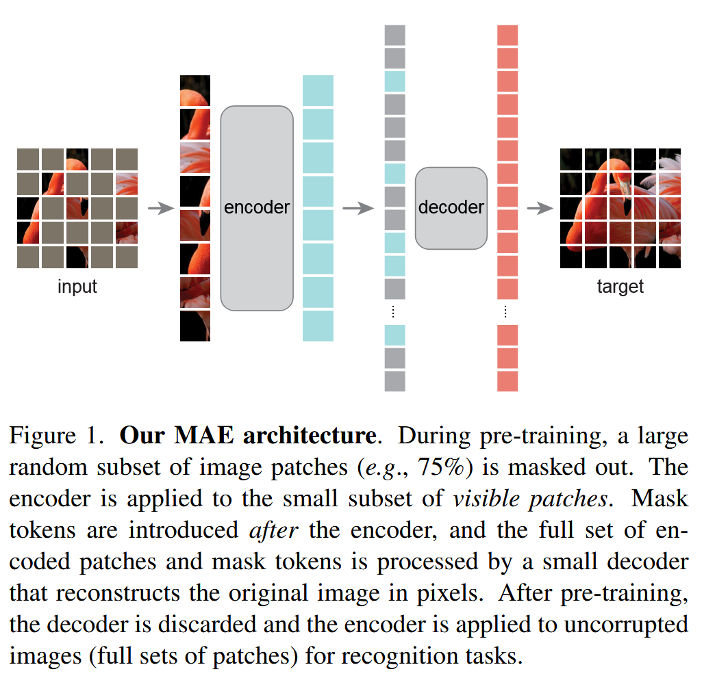
Source: Original Documents

masked autoencoders (MAE) are scalable self-supervised learners for computer vision High masking ratio + Asymmetric encoder-decoder를 결합해 representation quality와 computational efficiency를 동시에 얻는다.

ViT-L: 모델 아키텍처
MAE: 그 모델을 학습시키는 self-supervised pre-training 방법
MAE-pretrained ViT-L: MAE 방식으로 사전학습된 ViT-L

⇒ MAE는 masked patch를 encoder에서 완전히 제거하여 visible patch만 latent representation으로 만들고, 이후 decoder 단계에서 masked 위치에 mask token을 다시 넣어 전체 이미지를 복원한다.

- Decoder는 전체 token을 처리해야 하므로, encoder에서 얻은 계산 효율을 유지하기 위해 **encoder보다 lightweight하게 설계한다.**
- 다만 **reconstruction-specific processing을 담당할 충분한 capacity는 필요**하며, 이후 ablation에서 decoder depth에 따른 representation quality 차이를 검증한다.

두가지 접근을 통해 이를 구현함

비대칭적인 Encoder-Decoder 구조를 만들었는데, Encoder의 경우 오직 마스킹 되지 않은 보이는 패치들로만 동작하고 Decoder의 경우 경량화된 부분으로 latent representation과 mask token으로부터 재구성하는 구조다.

we develop an asymmetric encoder-decoder architecture, with an encoder that operates only on the visible subset of patches (without mask tokens), along with a lightweight decoder that reconstructs the original image from the latent representation and mask tokens.

- latent representation :
MAE의 encoder가 **보이는 패치(visible patches)**만 입력받아서 Transformer를 통과시킨 뒤 만들어낸 **고수준 feature representation**
    - `latent`는 쉽게 말하면 **직접 관측되는 픽셀이 아니라 모델 내부에서 학습된 숨겨진 표현이라는 뜻**
    - **무거운 encoder는 visible patch만 처리하고, mask token은 가벼운 decoder에서만 추가**하기 때문에 encoder의 계산량을 크게 줄일 수 있다.

입력 이미지의 상당 부분을 가리는 마스킹 비율 전략이 꽤 의미있는 self-supervisory task를 만들어준다.

Encoder에는 전체 패치의 작은 비율만 프로세싱하도록 해서 사전학습 시잔을 3배 이상으로 줄일 수 있었고 메모리 소비량도 줄였다. ⇒ Good Scalability로 이어짐

5. Result

ViT-Huge 모델과 같이 학습을 위해 많은 데이터를 필요로 하는 모델이 ImageNet-1K에 대해 학습하는데 더 향상된 generalization 성능을 보여주며 학습을 가능하게 했다.

또한 object detection, instance segmentation, semantic segmentation과 같은 과제에서 전이 학습되는 것에 평가해보았는데 이 masked 방식의 사전학습 접근이 기존의 supervised 방식으로 학습된 것 보다 더 좋은 결과를 보여주었고 scaling 하는데에도 이득을 얻는 것을 확인했다.

⇒ **저자들은 모델 크기를 키울수록 self-supervised pre-training의 이점이 커지는 이러한 scaling behavior가 NLP에서 관찰된 흐름과 유사하다고 본다.**


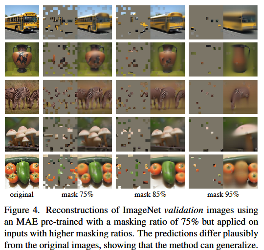
![Notion image](/notion-assets/reading-note-masked-autoencoders-are-scalable-vision-learners/3c114b84a0f2801ea472d8407dfd0afc.png)


Source: Original Document

ViT-Large와 비교한 결과

ViT-L trained from scratch
fine-tuned from baseline MAE

Notion image

→ ViT-L이 바로 supervised training을 하는 것은 그다지 중요하지 않았고 오히려 strong regularization 전략이 중요했다.

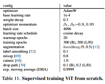
![Notion image](/notion-assets/reading-note-masked-autoencoders-are-scalable-vision-learners/3c514b84a0f280069838f39796bad908.png)


Source: Original Document

> ViT-L/H를 from scratch로 안정적으로 supervised train하기 위한 recipe

MAE pre-training 같은 사전학습을 전혀 하지 않고, ViT-L/H의 weight를 처음부터 초기화한 뒤 ImageNet-1K의 class label을 직접 사용해서 classification task로 end-to-end 학습했다

⇒ ViT-L은 overfitting하는 경향도 있고 사전학습을 진행하면 오히려 성능이 떨어지는 모습을 보였기에 MAE의 성능을 더 정확하게 비교하기 위해 강한 regularization을 진행했다.

⇒ 이렇게 해도 MAE의 성능이 더 높았다.

5.1. Comparisons with Previous Results

5.1.1. Comparisons with self-supervised methods

Notion image

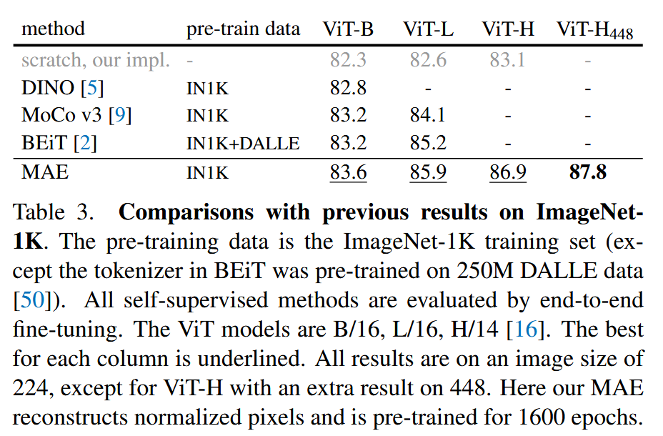
Source: Original Document

end-to-end fine-tuning으로 평가 진행
ViT-B에서는 모든 방법론이 비슷한 성능을 보였지만 ViT의 경우 방법론 간의 정확도 차이가 조금씩 커졌다. ⇒ 더 큰 모델의 challenge는 overfitting 방지 (MAE가 이 overfitting 방지에 좋은 성능을 보여주는게 아닐까? 하는거임)
BEiT 와 비교해서 MAE가 더 간단하고 더 빠른 동시에 더 정확한 모습을 보여준다.
또한 MAE의 경우 성능을 위해 1600 epoch로 사전학습을 진행했음에도 불구하고 다른 방법에 비해 더 빠르게 학습을 진행하였다.

5.1.2. Comparisons with supervised pre-training

ViT 기존 연구에 비롯할 때 ViT-L은 ImageNet-1K에 학습했을때 성능이 떨어졌다.

저자들도 supervised learning을 진행했지만 더 좋은 성능을 보여주긴 했지만 accuracy saturation 문제가 발생했다.

Source: Original Document

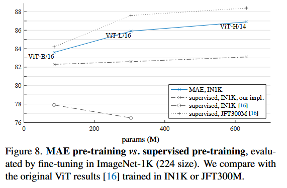
MAE 사전학습의 경우 IN1K만을 활용함에도 불구하고 더 좋은 일반화 성능을 보여준다.

> 같은 모델을 from scratch로 학습했을 때와 비교해서, **MAE pre-training을 거쳤을 때 얻는 성능 향상**폭이 ViT-B보다 ViT-L/H 같은 큰 모델에서 더 크다

이는 table 3에서의 정보를 통해 확인 가능하다


| 모델    | Supervised from scratch | MAE pre-training + FT | MAE의 gain  |
| ----- | ----------------------- | --------------------- | ---------- |
| ViT-B | 82.3                    | 83.6                  | **+1.3%p** |
| ViT-L | 82.6                    | 85.9                  | **+3.3%p** |
| ViT-H | 83.1                    | 86.9                  | **+3.8%p** |

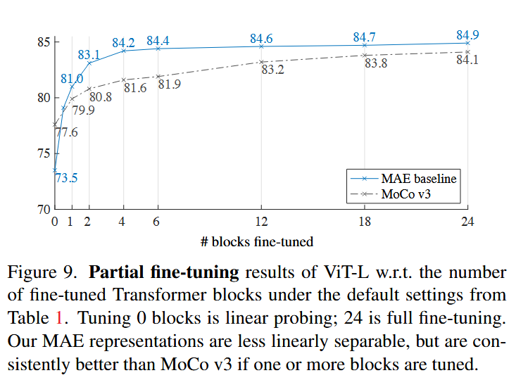
5.2. Partial Fine-tuning

Table 1에서도 나왔듯이 linear probing과 fine-tuning은 그렇게 큰 연관성이 없었다.
linear probing은 물론 지난 몇년간 (저자 기준) 인기있는 방법이었지만 가장 큰 한계점은 non-linear features에 대해 학습이 어렵다라는 것

⇒ 그래서 linear-probing 과정에서 last several layers를 fine-tuning하는 partial fine-tuning 방식을 시도했는데 그렇게 새로운 방법은 아니었다.

Notion image

Source: Original Document

0 block일때 linear probing, 24 blocks 일때 fine-tuning이다.
한 블럭만 fine-tuning을 진행했을때 꽤 큰 상승폭을 보였음 (7.5%p)

💡 여기서 말하는 블록이 무엇인가? MAE pre-training에 사용했던 decoder block 수가 아니라, pre-trained ViT-L encoder의 Transformer block 중 뒤쪽 몇 개를 supervised fine-tuning할 것인지

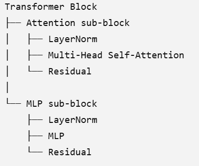
이런 구조의 블록이 24개 이어진게 ViT-L의 구조. 여기서 몇개의 블록까지 backpropagation을 진행하느냐? 학습을 반영할 것이냐가 이 단락에서 보고자하는 것이다.
마지막 블록의 절반만 fine-tune할때 (Transformer Block에서 MLP sub-block만 fine-tuning하고 attention sub-block은 freeze)는 linear probing보다 더 좋은 성능을 보였다. (79.1%)
MoCo v3과도 비교를 였는데 linear probing accuracy에서는 높은 성능을 보여주었지만 fine-tuning을 진행할수록 성능이 뒤처지는 모습이 보였다.

⇒ MAE representation은 linearly separable하지는 않지만 non-linear features에는 강하며 non-linear head가 조정되었을때 더 좋은 성과를 보인다.

그러면 MoCov3 representation과 MAE representation을 tSNE와 같이 시각화를 했다면 더 근거가 뒷받침 되지 않았을까?

Representation analysis: MAE가 MoCo v3보다 less linearly separable하지만 stronger non-linear feature를 학습한다는 주장은 partial fine-tuning 성능으로 뒷받침된다. 다만 frozen representation의 geometry를 t-SNE/UMAP 등으로 시각화하거나 linear vs. nonlinear probe를 추가했다면 두 representation의 차이를 더 직접적으로 분석할 수 있었을 것이다. 단, t-SNE 자체는 nonlinear projection이므로 linear separability의 정량적 근거로 사용할 수는 없다.

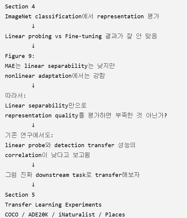
5.2. Transfer Learning Experiments

evaluate transfer learning in downstream tasks using the pre-trained models Mask R-CNN을 COCO에 대하여 fine-tuning하고 ViT backbone은 FPN을 활용하여 적용함

Mask R-CNN heads ├─ Bounding box prediction └─ Instance mask prediction

그렇기에 오직 Downstream task에 대한 pre-training 전략의 차이만 보기 때문에 pre-training 이후는 동일하게 작업

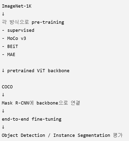
5.2.1. Object detection and segmentation

Notion image

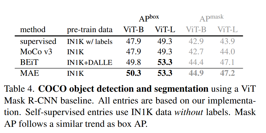
Source: Original Document

모든 실험 조건에서 MAE가 가장 우수한 성능을 보였다. 하지만 그렇다고 BEiT와 비교해서 그렇게 두드러지는 차이를 보이주지는 않는다.
- ⇒ BEiT는 Token base이고 MAE는 pixel base이기 때문에 완전히 우수하지는 않아도 더 간단한 원리와 구조로 동률의 성능을 낸다는 것 자체가 의미있는일.
model capacity를 더 키웠을떄 (ViT-B → ViT-L) classification과 동일하게 scalability 측면에서 더 좋은 성능을 보여준다.

1. MAE representation은 classification에만 좋은 것이 아니라 object detection과 instance segmentation으로도 잘 transfer된다. 2. 특히 ViT-B보다 ViT-L에서 supervised 대비 gain이 더 커서, MAE의 scaling benefit이 downstream transfer에서도 나타난다. 3. Linear probing에서는 강했던 MoCo v3보다 실제 detection transfer에서는 MAE가 훨씬 좋고, 복잡한 dVAE token을 쓰는 BEiT와도 같거나 더 좋은 성능을 보인다.

💡 Object Detection 성능은 어떻게 평가하는가?

예측 box와 정답 box가 얼마나 겹치는지 **IoU(Intersection over Union)**를 계산

특정 IoU threshold를 정해서 예측을 TP/FP로 판단합니다. 예를 들어 IoU ≥ 0.5라면 올바른 detection으로 보는 식.

Segmentation에서도 역시 IoU의 개념을 통해 P, N을 골라낸다.

Metric 무엇을 평가?
AP_box 객체의 bounding box 위치
AP_mask 객체의 실제 pixel-level 형태

Metric	무엇을 평가?
`AP_box`	객체의 bounding box 위치
`AP_mask`	객체의 실제 pixel-level 형태

5.2.2. Semantic segmentation

Notion image

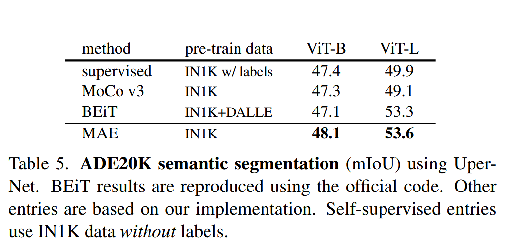
Source: Original Document

semantic segmentation에서도 역시 MAE가 좋은 성능을 보여준다.

💡 Semantic Segmentation에서는 어떻게 모델의 성능을 평가하는가?

Semantic segmentation은 이미지의 모든 pixel을 class로 분류한다.

모든 class에 대해 계산한 다음 평균냅니다.

$mIoU=\frac{1}{C}∑_{c=1}^CIoUc$

그래서 mIoU = mean Intersection over Union

5.2.3. Classification Tasks

Notion image

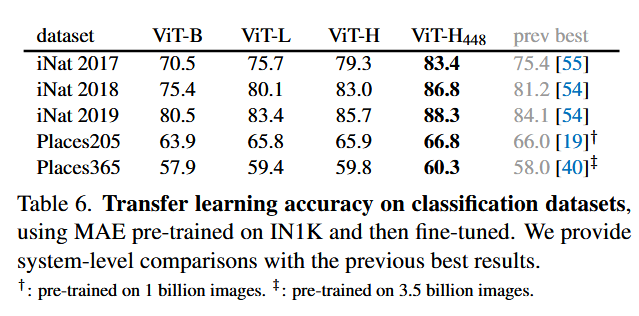
Source: Original Document

MAE representation이 다른 classification dataset에도 잘 transfer되는가?

MAE로 pre-training한 representation은 다른 classification dataset으로 transfer했을 때도 larger model의 capacity를 효과적으로 활용한다.

5.2.4. Pixels vs. tokens

Notion image

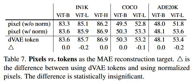
Source: Original Document

Reconstruction target으로 raw pixel, normalized pixel, dVAE token 중 무엇을 쓰는 것이 실제 downstream transfer에도 좋은가?

MAE reconstruction target으로 unnormalized pixel, normalized pixel, dVAE token을 비교했다. dVAE token은 unnormalized pixel보다 일부 개선되지만, normalized pixel과는 IN1K/COCO/ADE20K 전반에서 통계적으로 거의 차이가 없었다.
따라서 별도 tokenizer와 token prediction 없이 단순한 normalized pixel reconstruction만으로도 충분한 transfer representation을 얻을 수 있다.

6. Limitation

1. Reconstruction–Semantics Gap

Pixel reconstruction이라는 low-level pretext task가 왜 high-level semantic representation으로 이어지는지에 대한 설명은 아직 가설적이며, representation 자체에 대한 직접적인 분석이 부족하다.

2. Representation Analysis 부족

MAE가 MoCo v3보다 less linearly separable but stronger non-linear features라는 주장은 partial fine-tuning 결과를 기반으로 하지만, feature-space visualization이나 nonlinear probing 등으로 representation 구조를 직접 검증하지 않았다.

3. Empirical Design Dependency

75% random masking, decoder 구조, normalized pixel target 등의 핵심 설계는 실험적으로 결정되었으며 다른 dataset/task에서도 동일하게 최적인지는 확인되지 않았다.

4. Image-only Setting

Spatial redundancy에 초점을 맞춘 static image pre-training이므로 temporal redundancy와 motion을 포함하는 video representation으로의 일반화는 검증되지 않았다.